> ## Documentation Index
> Fetch the complete documentation index at: https://docs.domino.ai/llms.txt
> Use this file to discover all available pages before exploring further.
# AutoML Studio
Train, evaluate, and deploy machine learning models through a unified no-code interface.
## Overview
AutoML is a Domino extension that enables data scientists and domain experts to build, evaluate, and deploy machine learning models through a streamlined, no-code interface.
Powered by AutoGluon, AutoML automates the end-to-end model training pipeline - from data profiling and feature engineering through model selection, hyperparameter tuning, and ensembling - so you can go from raw data to a production-ready model in minutes.
AutoML provides two primary workflows:
* **Data Exploration:** Upload a dataset, review column statistics and distributions, examine correlations, assess data quality, and apply transformations before training.
* **Model Training:** Configure and run an AutoGluon training job that automatically trains multiple model types, ranks them on a leaderboard, and produces deployment-ready artifacts.
Exported models and notebooks should only be shared with authorized users.
You can access AutoML from the left navigation sidebar of any Domino project under the **Extensions** section.
## Get started
### Prerequisites
* A Domino project with the AutoML extension enabled.
* A dataset in CSV or Parquet format (maximum file size: 550 MB).
* Alternatively, a file stored in a mounted Domino Dataset.
### Access AutoML
1. Navigate to your Domino project.
2. In the left sidebar, scroll down to the **Extensions** section.
3. Click **AutoML**.
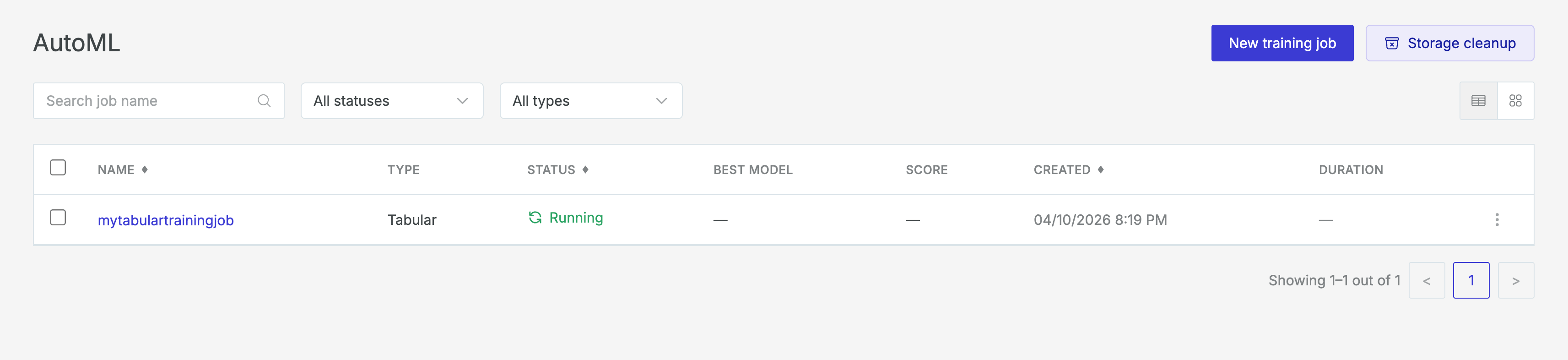
The AutoML landing page displays all existing training jobs with their name, type, status, best model, and creation date. From here you can start a new training job or explore your data.
Use the **Explore Data** button in the top-right corner of the AutoML landing page to profile and transform your data before creating a training job.
 ## Data Exploration
The Data Exploration tool lets you analyze data quality, distributions, and correlations, and prepare transformations before training a model.
To open it, click **Explore Data** from the AutoML landing page.
### Upload data
You can provide data in one of two ways:
* **Upload File:** Drag and drop (or click to browse) a CSV or Parquet file. The maximum file size is 550 MB.
* **Domino Dataset:** Select a file from a mounted Domino Dataset already connected to your project.
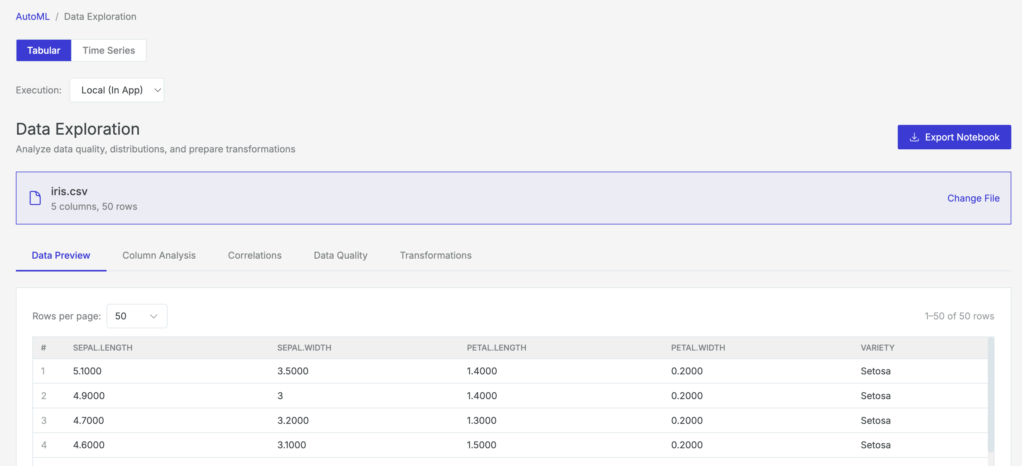
Once a file is loaded, Domino automatically profiles the data and takes you to the **Data Exploration** interface. The file name, column count, and row count are displayed at the top of the page. You can switch to a different file at any time by clicking **Change File**.
## Data Exploration
The Data Exploration tool lets you analyze data quality, distributions, and correlations, and prepare transformations before training a model.
To open it, click **Explore Data** from the AutoML landing page.
### Upload data
You can provide data in one of two ways:
* **Upload File:** Drag and drop (or click to browse) a CSV or Parquet file. The maximum file size is 550 MB.
* **Domino Dataset:** Select a file from a mounted Domino Dataset already connected to your project.
Once a file is loaded, Domino automatically profiles the data and takes you to the **Data Exploration** interface. The file name, column count, and row count are displayed at the top of the page. You can switch to a different file at any time by clicking **Change File**.
 ### Data Preview
The **Data Preview** tab shows a sample of your raw data in table format. You can browse columns and rows to get a quick sense of the dataset’s structure and values. Use the **Rows per page** control to adjust how many rows are displayed at a time.
### Data Preview
The **Data Preview** tab shows a sample of your raw data in table format. You can browse columns and rows to get a quick sense of the dataset’s structure and values. Use the **Rows per page** control to adjust how many rows are displayed at a time.
 ### Column Analysis
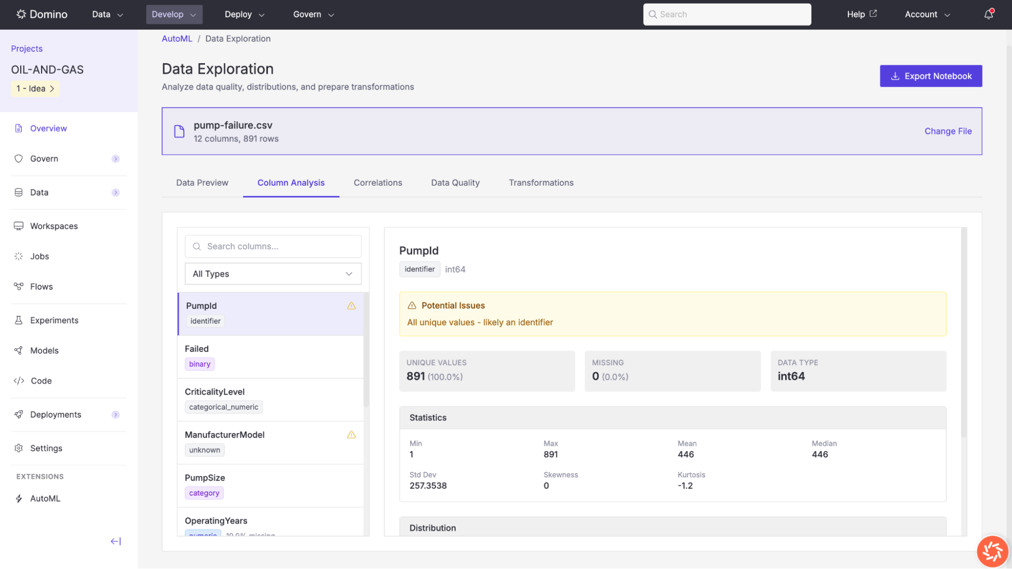
The **Column Analysis** tab provides detailed profiling information for each column in your dataset. Select a column from the list on the left to view its profile on the right.
AutoML automatically detects each column’s semantic type, displayed as a colored tag beneath the column name. Detected types include:
| Type | Description | Color |
| ------------------------ | --------------------------------------------------------------------------------------------------------------------------------------------------------------------------------------------------------------------------- | ------ |
| **numeric** | A column containing continuous numeric values (integers or floats). | Blue |
| **monetary** | A numeric column identified by name patterns related to financial values (e.g., `price`, `cost`, `amount`, `revenue`, `salary`). | Blue |
| **binary** | A numeric column with exactly two distinct values, commonly used as a classification target. | Purple |
| **category** | A column with a moderate number of distinct text or object values, or identified by name patterns (e.g., `type`, `class`, `status`, `group`). | Purple |
| **categorical\_numeric** | A numeric column with fewer than 20 distinct values representing less than 5% of the total rows, treated as a categorical feature. | Purple |
| **datetime** | A column containing date or timestamp values, detected by data type or name patterns (e.g., `date`, `time`, `timestamp`, `created`, `updated`). | Green |
| **text** | A column containing long text strings (average length > 100 characters), or identified by name patterns (e.g., `description`, `comment`, `note`). | Orange |
| **identifier** | A column whose values are likely unique row identifiers, detected by name patterns (e.g., `id`, `uuid`, `guid`) or high cardinality. Identifiers are flagged with a warning and should typically be excluded from training. | Gray |
| **boolean** | A column containing true/false values, detected by data type or name patterns (e.g., `is_`, `has_`, `flag`). | Gray |
| **unknown** | A column whose type could not be confidently determined. Review these columns manually before training. | Gray |
Additional types are detected but displayed with default styling:
* **email:** Columns with email-related names
* **phone:** Columns with phone-related names
* **url:** Columns with URL-related names
* **latitude/longitude:** Geographic coordinate columns
* **percentage:** Columns with percentage-related names (e.g., `percent`, `pct`, `ratio`, `rate`)
* **name:** Columns with name-related patterns (e.g., `name`, `title`, `label`)
* **count:** Columns with count-related names (e.g., `count`, `num`, `qty`, `quantity`)
For each selected column, the following information is displayed:
* **Potential Issues:** Warnings such as `High cardinality – may be an identifier`, `High missing rate`, or `Constant or near-constant column`.
* **Unique Values:** The count and percentage of distinct values.
* **Missing:** The count and percentage of null or missing entries.
* **Data Type:** The underlying Pandas data type (e.g., `int64`, `object`, `float64`).
* **Statistics:** For numeric columns: `min`, `max`, `mean`, `median`, `standard deviation`, `skewness`, and `kurtosis`.
* **Distribution:** A histogram for numeric columns, or a bar chart of top values for categorical columns showing the count and percentage for each category.
### Column Analysis
The **Column Analysis** tab provides detailed profiling information for each column in your dataset. Select a column from the list on the left to view its profile on the right.
AutoML automatically detects each column’s semantic type, displayed as a colored tag beneath the column name. Detected types include:
| Type | Description | Color |
| ------------------------ | --------------------------------------------------------------------------------------------------------------------------------------------------------------------------------------------------------------------------- | ------ |
| **numeric** | A column containing continuous numeric values (integers or floats). | Blue |
| **monetary** | A numeric column identified by name patterns related to financial values (e.g., `price`, `cost`, `amount`, `revenue`, `salary`). | Blue |
| **binary** | A numeric column with exactly two distinct values, commonly used as a classification target. | Purple |
| **category** | A column with a moderate number of distinct text or object values, or identified by name patterns (e.g., `type`, `class`, `status`, `group`). | Purple |
| **categorical\_numeric** | A numeric column with fewer than 20 distinct values representing less than 5% of the total rows, treated as a categorical feature. | Purple |
| **datetime** | A column containing date or timestamp values, detected by data type or name patterns (e.g., `date`, `time`, `timestamp`, `created`, `updated`). | Green |
| **text** | A column containing long text strings (average length > 100 characters), or identified by name patterns (e.g., `description`, `comment`, `note`). | Orange |
| **identifier** | A column whose values are likely unique row identifiers, detected by name patterns (e.g., `id`, `uuid`, `guid`) or high cardinality. Identifiers are flagged with a warning and should typically be excluded from training. | Gray |
| **boolean** | A column containing true/false values, detected by data type or name patterns (e.g., `is_`, `has_`, `flag`). | Gray |
| **unknown** | A column whose type could not be confidently determined. Review these columns manually before training. | Gray |
Additional types are detected but displayed with default styling:
* **email:** Columns with email-related names
* **phone:** Columns with phone-related names
* **url:** Columns with URL-related names
* **latitude/longitude:** Geographic coordinate columns
* **percentage:** Columns with percentage-related names (e.g., `percent`, `pct`, `ratio`, `rate`)
* **name:** Columns with name-related patterns (e.g., `name`, `title`, `label`)
* **count:** Columns with count-related names (e.g., `count`, `num`, `qty`, `quantity`)
For each selected column, the following information is displayed:
* **Potential Issues:** Warnings such as `High cardinality – may be an identifier`, `High missing rate`, or `Constant or near-constant column`.
* **Unique Values:** The count and percentage of distinct values.
* **Missing:** The count and percentage of null or missing entries.
* **Data Type:** The underlying Pandas data type (e.g., `int64`, `object`, `float64`).
* **Statistics:** For numeric columns: `min`, `max`, `mean`, `median`, `standard deviation`, `skewness`, and `kurtosis`.
* **Distribution:** A histogram for numeric columns, or a bar chart of top values for categorical columns showing the count and percentage for each category.
 ### Correlations
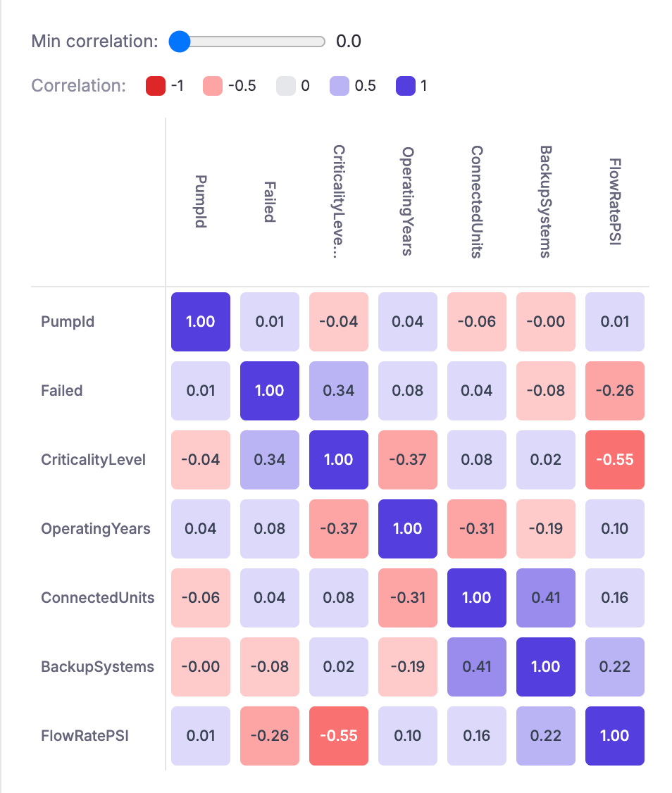
The **Correlations** tab displays a correlation matrix heatmap for all numeric columns in the dataset. Correlation values range from −1 (strong negative correlation) to +1 (strong positive correlation), with color coding to highlight the strength and direction of each relationship.
Use the **Min correlation** slider to filter out weak correlations and focus on the strongest relationships. This view is helpful for identifying multicollinearity between features and understanding which variables are most associated with your target column.
### Correlations
The **Correlations** tab displays a correlation matrix heatmap for all numeric columns in the dataset. Correlation values range from −1 (strong negative correlation) to +1 (strong positive correlation), with color coding to highlight the strength and direction of each relationship.
Use the **Min correlation** slider to filter out weak correlations and focus on the strongest relationships. This view is helpful for identifying multicollinearity between features and understanding which variables are most associated with your target column.
 ### Data Quality
The **Data Quality** tab gives you an at-a-glance assessment of your dataset’s readiness for model training. It includes the following sections:
* **Missing Values by Column:** A horizontal bar chart showing the number and percentage of missing values for each column that has any. Columns are color-coded by severity: green for less than 5% missing, orange for 5–20%, yellow for 20–50%, and red for more than 50%.
* **Missing Value Pattern:** A compact visual representation of where missing values occur across columns, helping you identify whether missingness is concentrated or scattered.
* **Warnings:** Issues that could affect training quality. For example, `Small dataset – consider using best_quality preset for better results`.
* **Recommendations:** Actionable suggestions to improve model performance. These are tagged by priority (high or medium) and category (Target, Preprocessing). Examples include:
* Potential binary classification targets (e.g., `Failed`, `PumpSize`).
* Potential multiclass classification targets (e.g., `CriticalityLevel`, `ConnectedUnits`, `BackupSystems`).
* Consider dropping or imputing columns with more than 30% missing values (e.g., `WellSector`).
### Data Quality
The **Data Quality** tab gives you an at-a-glance assessment of your dataset’s readiness for model training. It includes the following sections:
* **Missing Values by Column:** A horizontal bar chart showing the number and percentage of missing values for each column that has any. Columns are color-coded by severity: green for less than 5% missing, orange for 5–20%, yellow for 20–50%, and red for more than 50%.
* **Missing Value Pattern:** A compact visual representation of where missing values occur across columns, helping you identify whether missingness is concentrated or scattered.
* **Warnings:** Issues that could affect training quality. For example, `Small dataset – consider using best_quality preset for better results`.
* **Recommendations:** Actionable suggestions to improve model performance. These are tagged by priority (high or medium) and category (Target, Preprocessing). Examples include:
* Potential binary classification targets (e.g., `Failed`, `PumpSize`).
* Potential multiclass classification targets (e.g., `CriticalityLevel`, `ConnectedUnits`, `BackupSystems`).
* Consider dropping or imputing columns with more than 30% missing values (e.g., `WellSector`).
 ### Transformations
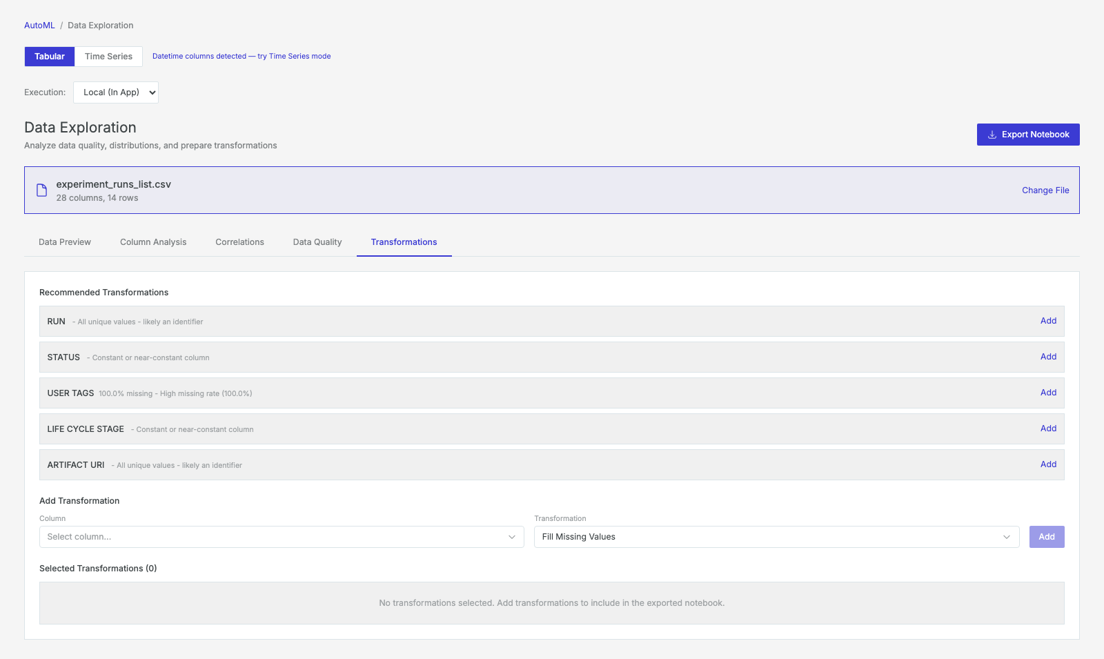
The **Transformations** tab lets you define preprocessing steps that will be applied to the dataset before model training. AutoML analyzes your data and suggests recommended transformations based on detected issues.
**Recommended transformations**
AutoML may recommend transformations for columns with the following issues:
* **Identifier columns:** Columns where all values are unique and are likely row identifiers (e.g., `PumpId`). *Recommended action:* drop the column.
* **High cardinality:** Columns that may be identifiers due to a very large number of unique values (e.g., `ManufacturerModel`). *Recommended action:* review and potentially drop.
* **Missing values:** Columns with a significant percentage of null values (e.g., `OperatingYears at 19.9% missing`). *Recommended action:* fill missing values.
* **Extreme outliers:** Numeric columns with extreme values detected (e.g., `FlowRatePSI with 6.9% outliers`). *Recommended action:* clip or remove outliers.
* **High missing rate:** Columns with a very high percentage of missing data (e.g., `WellSector at 77% missing`). *Recommended action:* drop the column.
Click **Add** next to any recommended transformation to include it. You can also create custom transformations by selecting a column and a transformation type (e.g., `Fill Missing Values`) from the dropdown controls at the bottom of the page.
All selected transformations appear in the **Selected Transformations** list. Transformations are included in the exported notebook and can be reviewed and modified in code.
### Transformations
The **Transformations** tab lets you define preprocessing steps that will be applied to the dataset before model training. AutoML analyzes your data and suggests recommended transformations based on detected issues.
**Recommended transformations**
AutoML may recommend transformations for columns with the following issues:
* **Identifier columns:** Columns where all values are unique and are likely row identifiers (e.g., `PumpId`). *Recommended action:* drop the column.
* **High cardinality:** Columns that may be identifiers due to a very large number of unique values (e.g., `ManufacturerModel`). *Recommended action:* review and potentially drop.
* **Missing values:** Columns with a significant percentage of null values (e.g., `OperatingYears at 19.9% missing`). *Recommended action:* fill missing values.
* **Extreme outliers:** Numeric columns with extreme values detected (e.g., `FlowRatePSI with 6.9% outliers`). *Recommended action:* clip or remove outliers.
* **High missing rate:** Columns with a very high percentage of missing data (e.g., `WellSector at 77% missing`). *Recommended action:* drop the column.
Click **Add** next to any recommended transformation to include it. You can also create custom transformations by selecting a column and a transformation type (e.g., `Fill Missing Values`) from the dropdown controls at the bottom of the page.
All selected transformations appear in the **Selected Transformations** list. Transformations are included in the exported notebook and can be reviewed and modified in code.
 ### Export a Notebook
At any point during data exploration, you can click the **Export Notebook** button in the top-right corner to download a Jupyter notebook that contains all of your data profiling results and any transformations you have selected.
This notebook can be opened in a Domino Workspace for further analysis or custom preprocessing.
## AutoML model training
AutoML model training uses AutoGluon to automatically train, tune, and rank multiple machine learning models. The training job wizard guides you through four steps: selecting your data source, choosing a model type, configuring training parameters, and reviewing your settings before launch.
To begin, click **New training job** from the AutoML landing page.
### Step 1: Select a data source
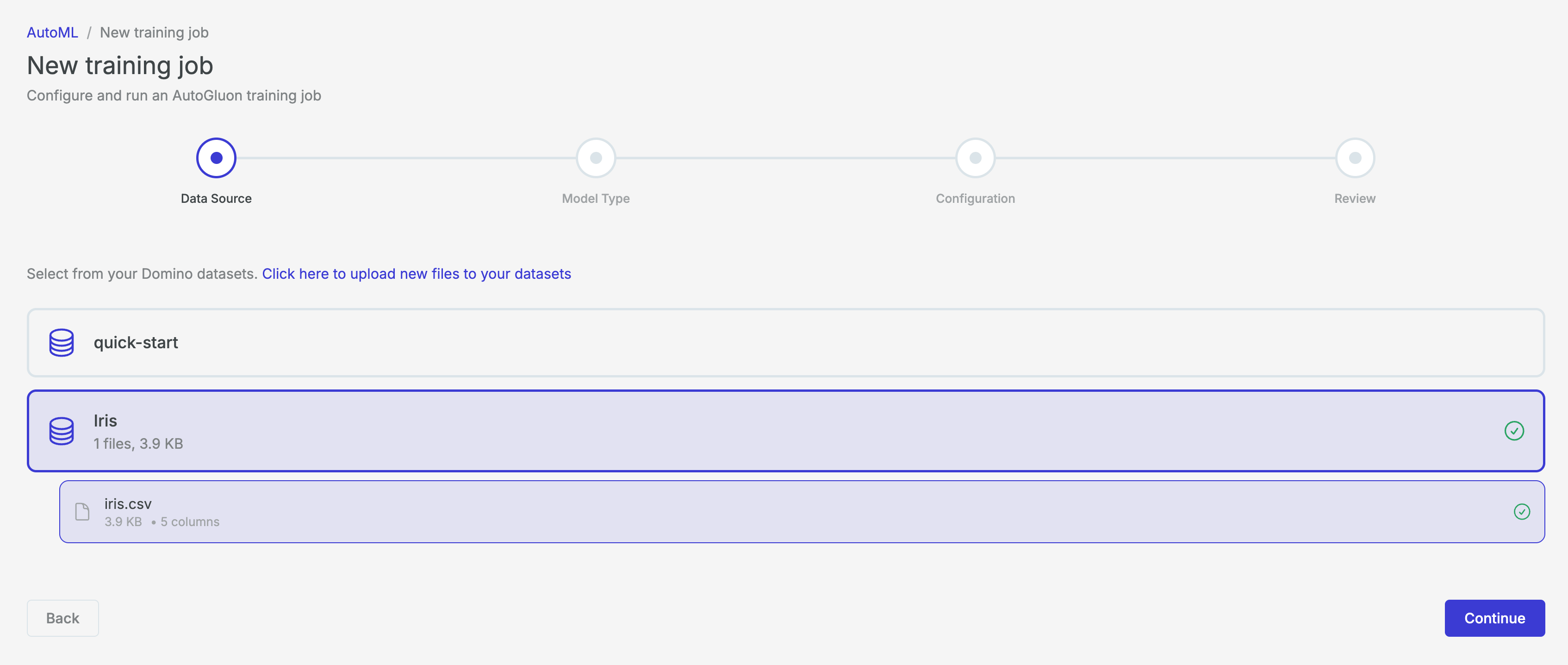
Select the dataset you want to use for training. As with Data Exploration, you can either upload a CSV or Parquet file (up to 550 MB) or select a file from a mounted Domino Dataset.
Once your file is loaded, click **Continue** to proceed.
### Export a Notebook
At any point during data exploration, you can click the **Export Notebook** button in the top-right corner to download a Jupyter notebook that contains all of your data profiling results and any transformations you have selected.
This notebook can be opened in a Domino Workspace for further analysis or custom preprocessing.
## AutoML model training
AutoML model training uses AutoGluon to automatically train, tune, and rank multiple machine learning models. The training job wizard guides you through four steps: selecting your data source, choosing a model type, configuring training parameters, and reviewing your settings before launch.
To begin, click **New training job** from the AutoML landing page.
### Step 1: Select a data source
Select the dataset you want to use for training. As with Data Exploration, you can either upload a CSV or Parquet file (up to 550 MB) or select a file from a mounted Domino Dataset.
Once your file is loaded, click **Continue** to proceed.
 ### Step 2: Select a model type
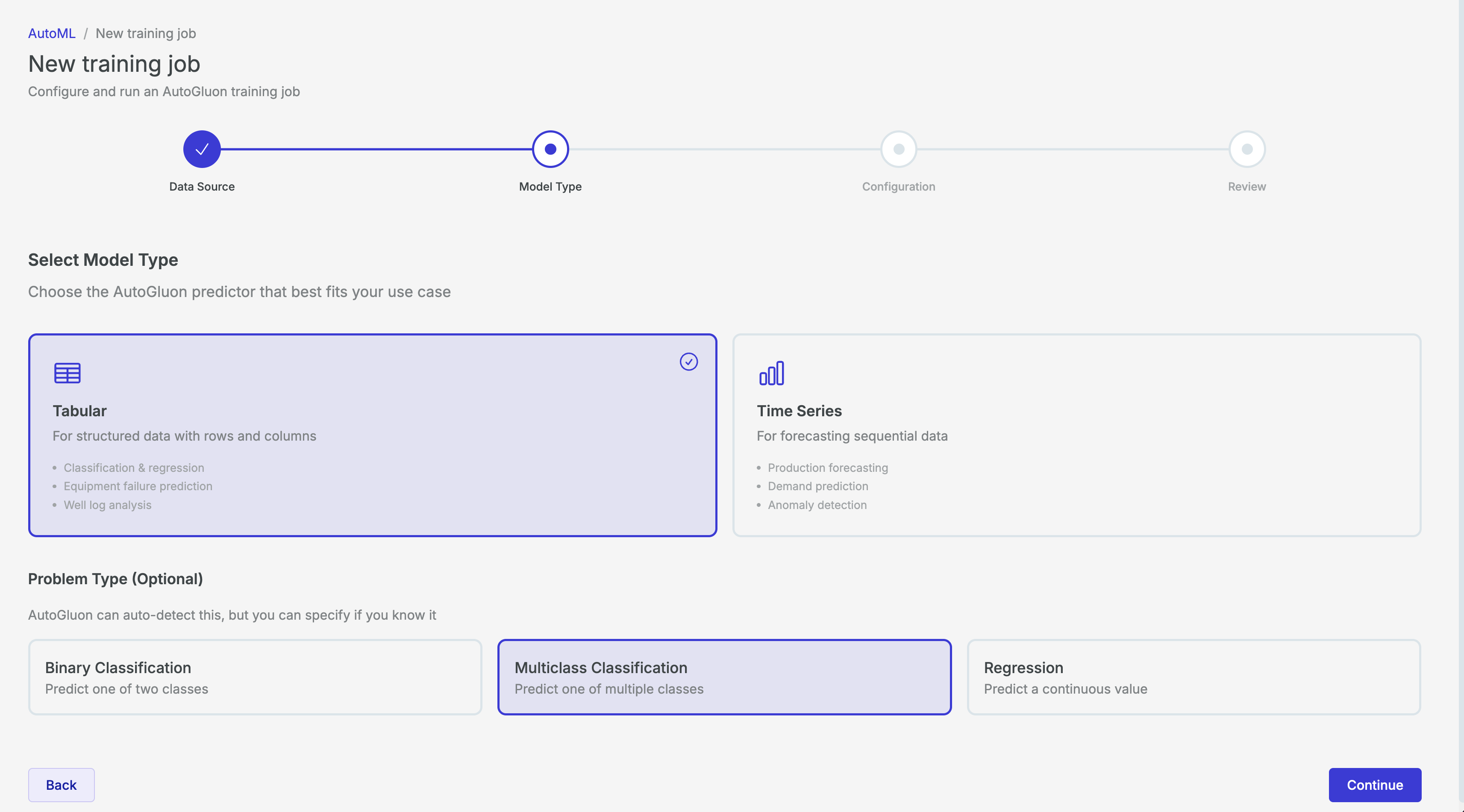
Choose the AutoGluon predictor that best fits your use case. Three model types are available:
| Model type | Description | Example use cases |
| --------------- | ---------------------------------------------------------------------------------------- | ------------------------------------------------------------------------------- |
| **Tabular** | For structured data with rows and columns. Supports classification and regression tasks. | Classification and regression, equipment failure prediction, well log analysis. |
| **Time Series** | For forecasting sequential data where observations are ordered over time. | Production forecasting, demand prediction, anomaly detection. |
| **Multimodal** | For mixed data types that combine images, text, and tabular data. | Seismic interpretation, document analysis, image + metadata. |
**Problem Type (Optional)**
AutoGluon can auto-detect the problem type from your target column, but you can also specify it explicitly:
| Problem type | Description |
| ----------------------------- | ----------------------------------------------------------------------- |
| **Binary Classification** | Predict one of two classes (e.g., `Failed: 0 or 1`). |
| **Multiclass Classification** | Predict one of multiple classes (e.g., `CriticalityLevel: 1, 2, or 3`). |
| **Regression** | Predict a continuous value (e.g., `FlowRatePSI`). |
Click **Continue** to proceed to configuration.
### Step 2: Select a model type
Choose the AutoGluon predictor that best fits your use case. Three model types are available:
| Model type | Description | Example use cases |
| --------------- | ---------------------------------------------------------------------------------------- | ------------------------------------------------------------------------------- |
| **Tabular** | For structured data with rows and columns. Supports classification and regression tasks. | Classification and regression, equipment failure prediction, well log analysis. |
| **Time Series** | For forecasting sequential data where observations are ordered over time. | Production forecasting, demand prediction, anomaly detection. |
| **Multimodal** | For mixed data types that combine images, text, and tabular data. | Seismic interpretation, document analysis, image + metadata. |
**Problem Type (Optional)**
AutoGluon can auto-detect the problem type from your target column, but you can also specify it explicitly:
| Problem type | Description |
| ----------------------------- | ----------------------------------------------------------------------- |
| **Binary Classification** | Predict one of two classes (e.g., `Failed: 0 or 1`). |
| **Multiclass Classification** | Predict one of multiple classes (e.g., `CriticalityLevel: 1, 2, or 3`). |
| **Regression** | Predict a continuous value (e.g., `FlowRatePSI`). |
Click **Continue** to proceed to configuration.
 ### Step 3: Configure Training
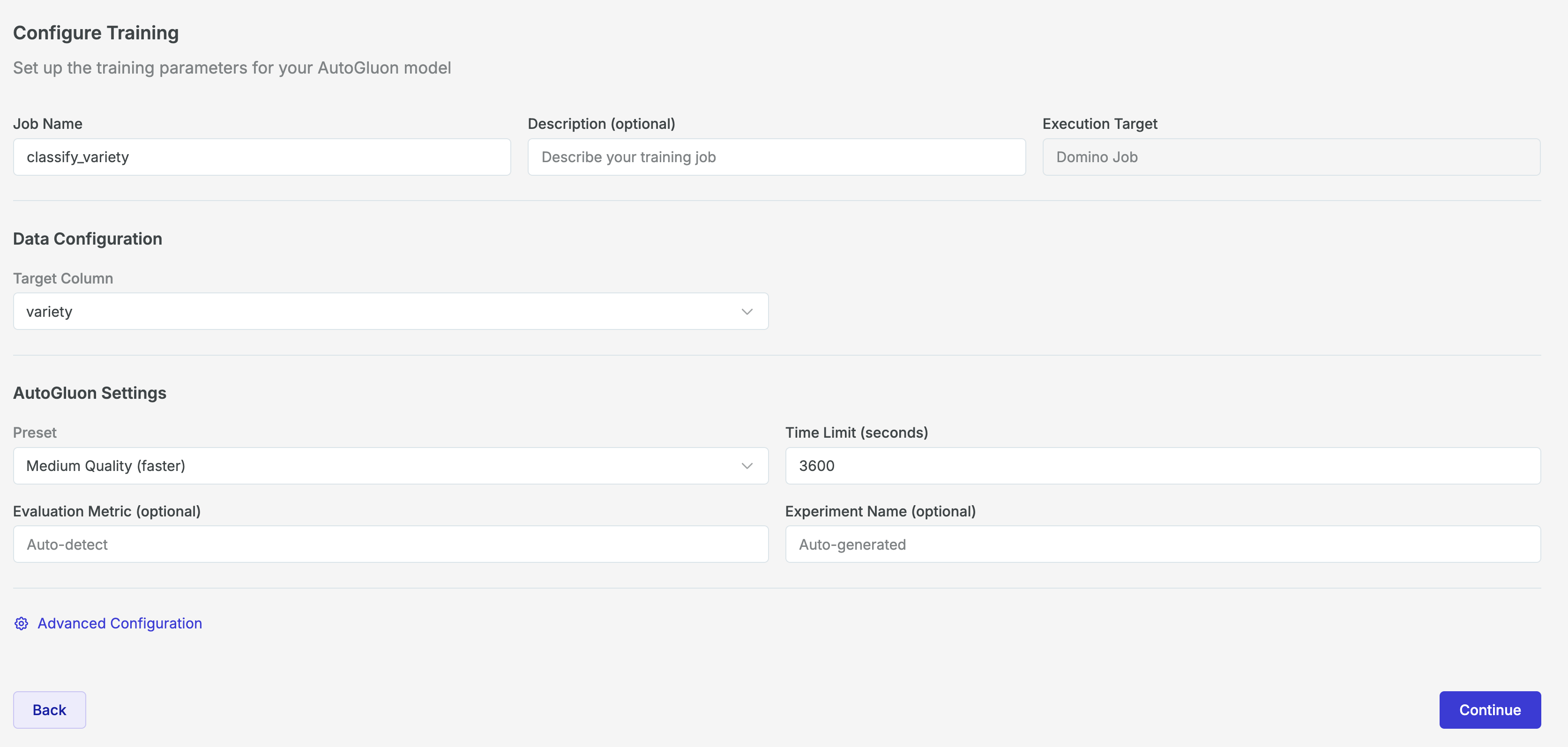
The configuration step lets you define your training job’s name, target column, and AutoGluon-specific settings.
#### Basic configuration
| Setting | Description |
| -------------------------- | ---------------------------------------------------------------------------------------------------------------- |
| **Job Name** | A descriptive name for this training run (e.g., `My training job`). |
| **Description (optional)** | A free-text description to help you identify this job later. |
| **Target Column** | The column in your dataset that the model should predict. Select it from the dropdown list of available columns. |
#### AutoGluon settings
| Setting | Description |
| -------------------------------- | --------------------------------------------------------------------------------------------------------------------------------------------------------------------------------------------------------------- |
| **Preset** | Controls the trade-off between model quality and training speed. Options include `Medium Quality (Faster)`, `Best Quality`, and others. `Medium Quality (Faster)` is the default. |
| **Time Limit (seconds)** | Maximum wall-clock time (in seconds) for the entire training run. Default: `3600 (1 hour)`. AutoGluon will train as many models as possible within this limit. |
| **Evaluation Metric (optional)** | The metric used to rank models on the leaderboard. Set to `Auto-detect` by default, which chooses an appropriate metric based on the problem type (e.g., `accuracy` for classification, `RMSE` for regression). |
| **Experiment Name (optional)** | An optional Domino Experiment name for tracking this run. If left blank, a name is auto-generated. |
### Step 3: Configure Training
The configuration step lets you define your training job’s name, target column, and AutoGluon-specific settings.
#### Basic configuration
| Setting | Description |
| -------------------------- | ---------------------------------------------------------------------------------------------------------------- |
| **Job Name** | A descriptive name for this training run (e.g., `My training job`). |
| **Description (optional)** | A free-text description to help you identify this job later. |
| **Target Column** | The column in your dataset that the model should predict. Select it from the dropdown list of available columns. |
#### AutoGluon settings
| Setting | Description |
| -------------------------------- | --------------------------------------------------------------------------------------------------------------------------------------------------------------------------------------------------------------- |
| **Preset** | Controls the trade-off between model quality and training speed. Options include `Medium Quality (Faster)`, `Best Quality`, and others. `Medium Quality (Faster)` is the default. |
| **Time Limit (seconds)** | Maximum wall-clock time (in seconds) for the entire training run. Default: `3600 (1 hour)`. AutoGluon will train as many models as possible within this limit. |
| **Evaluation Metric (optional)** | The metric used to rank models on the leaderboard. Set to `Auto-detect` by default, which chooses an appropriate metric based on the problem type (e.g., `accuracy` for classification, `RMSE` for regression). |
| **Experiment Name (optional)** | An optional Domino Experiment name for tracking this run. If left blank, a name is auto-generated. |
 #### Advanced Configuration
Click **Advanced Configuration** to access fine-grained controls organized across multiple tabs. Available tabs vary based on the selected model type.
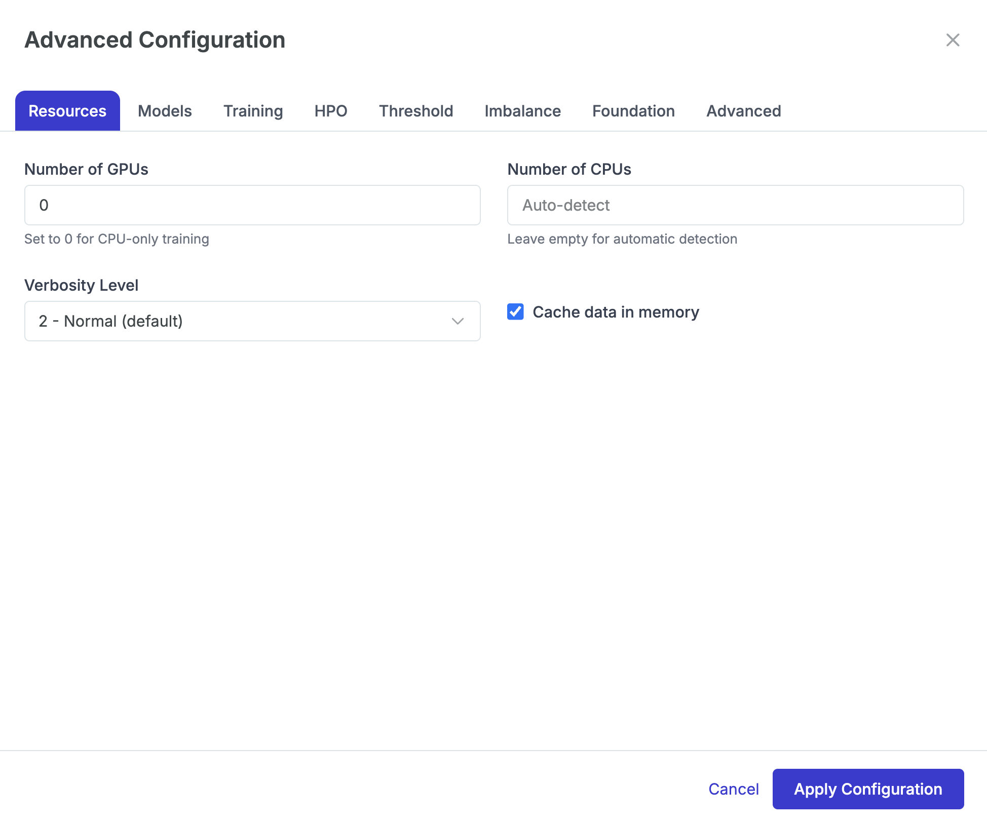
**Resources**
Configure compute resources allocated to the training job.
| Setting | Description |
| ------------------- | ------------------------------------------------------------------------------------------------------------------ |
| **Number of GPUs** | Set to `0` for CPU-only training. Increase for GPU-accelerated models. |
| **Number of CPUs** | Leave empty for automatic detection based on available hardware. |
| **Verbosity Level** | Controls logging detail: `0` (Silent), `1` (Errors only), `2` (Normal), `3` (Detailed), `4` (Debug). Default: `2`. |
| **Cache Data** | Cache data in memory for faster training. Enabled by default. |
**Models**
Select or exclude specific model families from the training run.
| Setting | Description |
| ------------------------ | -------------------------------------------------------------------------------------------------------------------------------------------------------------------------------------------------------------------------------------- |
| **Excluded Model Types** | Click to exclude model types from training (highlighted in red). Available models: LightGBM, CatBoost, XGBoost, Random Forest, Extra Trees, K-Nearest Neighbors, Linear Regression, Neural Network (PyTorch), Neural Network (FastAI). |
| **Bagging Folds** | Number of folds for bagging (2–10). Set to `Auto` by default. |
| **Stack Levels** | Number of stacking levels (0–3). Higher values increase ensemble complexity. |
| **Auto Stack** | Automatically determine optimal stacking configuration. |
**Training**
Fine-tune the training process.
| Setting | Description |
| -------------------------------- | --------------------------------------------------------------------------------------------------------------------------- |
| **Holdout Fraction** | Fraction of data reserved for validation (0.01–0.5). Typically 0.1–0.2. Set to `Auto` by default. |
| **Inference Time Limit (s/row)** | Maximum inference time per row in seconds. Leave blank for no limit. |
| **Calibrate Probabilities** | Calibrate predicted probabilities for better reliability. Useful when probability outputs will be used for decision-making. |
| **Refit on Full Data** | After training, refit the best models on the full dataset (training + validation) for maximum performance. |
| **Use Bag Holdout** | Use a separate holdout for bagged models, which can improve ensemble quality. |
**Hyperparameter Optimization (HPO)**
Enable and configure hyperparameter tuning. When enabled, AutoGluon searches over hyperparameter combinations for each model family.
| Setting | Description |
| ---------------------------- | --------------------------------------------------------------------------- |
| **Enable HPO** | Toggle hyperparameter optimization on/off. |
| **HPO Scheduler** | Local (single machine) or Ray (distributed across multiple workers). |
| **Search Algorithm** | Auto (recommended), Random Search, Bayesian Optimization, or Grid Search. |
| **Number of Trials** | More trials = better results but longer training (1–100). Default: `10`. |
| **Max Iterations per Trial** | Maximum training iterations for each trial. Leave blank for *auto*. |
| **Grace Period** | Minimum iterations before early stopping can occur (ASHA scheduler). |
| **Reduction Factor** | Factor by which to reduce the number of trials at each rung. Typically `3`. |
Per-Model Hyperparameters: Override default hyperparameters for specific model types (LightGBM, XGBoost, CatBoost, Neural Network) using JSON format.
**Threshold**
For binary classification tasks, optimize the decision threshold.
| Setting | Description |
| -------------------------------- | ---------------------------------------------------------------------------------------------------------------------------- |
| **Enable Threshold Calibration** | Find optimal decision threshold instead of using the default `0.5`. |
| **Optimization Metric** | Metric to optimize: `Balanced Accuracy` (default), `F1 Score`, `Precision`, `Recall`, or `Matthews Correlation Coefficient`. |
| **Thresholds to Try** | Number of threshold values to evaluate (10–1000). Default: `100`. |
**Imbalance**
Configure how AutoGluon handles class imbalance.
| Setting | Description |
| ------------------------ | ------------------------------------------------------------------------------------------------------------------------------------------------------------------------------- |
| **Imbalance Strategy** | None (default), Oversample (duplicate minority class), Undersample (reduce majority class), SMOTE (synthetic minority oversampling), or Focal Loss (down-weight easy examples). |
| **Sample Weight Column** | Name of a column containing sample weights for weighted training. |
**Foundation**
Options for foundation model-based approaches.
| Setting | Description |
| --------------------------------- | ------------------------------------------------------------------------------------------------------------------------------------------ |
| **Use Tabular Foundation Models** | Include `TabPFN` and other foundation models in training. |
| **Foundation Model Preset** | None (use with other models), Zero-shot (instant predictions without training), or Zero-shot + HPO (optimize foundation model parameters). |
| **Dynamic Stacking** | Use dynamic stacking for adaptive ensemble configurations. |
| **Pseudo-Labeling** | Enable semi-supervised learning with unlabeled data. Requires specifying an unlabeled data path. |
| **Drop Unique Features** | Automatically drop high-cardinality unique features (like IDs). |
**Advanced**
Additional low-level AutoGluon parameters for experienced users.
| Setting | Description |
| -------------------------------- | ------------------------------------------------------------------------------------------------------- |
| **Enable Distillation** | Transfer knowledge from the ensemble to a single faster model for deployment. |
| **Distillation Time Limit** | Time allocated for distillation (seconds). Leave blank for *auto*. |
| **Include Only Specific Models** | Whitelist specific model types to include (overrides excluded models). Selected models appear in green. |
| **Bagging Sets** | Number of complete bagging sets (increases diversity). |
| **Use Refit as Best** | Use the refitted model as the final predictor. |
**Time Series**
Configure time series-specific settings.
| Setting | Description |
| ---------------------- | ------------------------------------------------------------------------------------------------------------------------------------------------------------------------------- |
| **Frequency** | Data frequency: `Auto-detect`, `Daily`, `Weekly`, `Monthly`, `Hourly`, `Minutely`, `Quarterly`, or `Yearly`. |
| **Target Scaler** | Scaling method for target values: `Default`, `Mean Absolute`, `Standard`, `Min-Max`, or `No Scaling`. |
| **Use Chronos** | Enable Amazon’s Chronos foundation model for time series forecasting. |
| **Chronos Model Size** | Model size when Chronos is enabled: `Tiny` (8M params), `Mini` (20M), `Small` (46M), `Base` (200M), or `Large` (710M). Larger models are more accurate but require more memory. |
| **Enable Ensemble** | Combine multiple time series models into an ensemble. Enabled by default. |
**Multimodal**
Configure multimodal-specific settings for combined image, text, and tabular data.
| Setting | Description |
| ------------------- | -------------------------------------------------------------------------------------------------------------- |
| **Text Backbone** | Pre-trained text model (e.g., `google/electra-base-discriminator`). |
| **Image Backbone** | Pre-trained image model (e.g., `swin_base_patch4_window7_224`). |
| **Max Text Length** | Maximum token length for text inputs (32–2048). Default: `512`. |
| **Image Size** | Input image size in pixels (32–512). Default: `224`. |
| **Batch Size** | Training batch size. Leave blank for *auto*. |
| **Max Epochs** | Maximum training epochs. Leave blank for *auto*. |
| **Learning Rate** | Model learning rate. Leave blank for *auto*. |
| **Fusion Method** | How to combine modalities: `Late Fusion` (combine at prediction) or `Early Fusion` (combine at feature level). |
**Summary of tabs availability by model type:**
| Tab | Tabular | Time Series | Multimodal |
| --------------- | ------- | ----------- | ---------- |
| **Resources** | ✓ | ✓ | ✓ |
| **Models** | ✓ | - | - |
| **Training** | ✓ | - | - |
| **HPO** | ✓ | - | - |
| **Threshold** | ✓ | - | - |
| **Imbalance** | ✓ | - | - |
| **Foundation** | ✓ | - | - |
| **Advanced** | ✓ | - | - |
| **Time Series** | - | ✓ | - |
| **Multimodal** | - | - | ✓ |
#### Advanced Configuration
Click **Advanced Configuration** to access fine-grained controls organized across multiple tabs. Available tabs vary based on the selected model type.
**Resources**
Configure compute resources allocated to the training job.
| Setting | Description |
| ------------------- | ------------------------------------------------------------------------------------------------------------------ |
| **Number of GPUs** | Set to `0` for CPU-only training. Increase for GPU-accelerated models. |
| **Number of CPUs** | Leave empty for automatic detection based on available hardware. |
| **Verbosity Level** | Controls logging detail: `0` (Silent), `1` (Errors only), `2` (Normal), `3` (Detailed), `4` (Debug). Default: `2`. |
| **Cache Data** | Cache data in memory for faster training. Enabled by default. |
**Models**
Select or exclude specific model families from the training run.
| Setting | Description |
| ------------------------ | -------------------------------------------------------------------------------------------------------------------------------------------------------------------------------------------------------------------------------------- |
| **Excluded Model Types** | Click to exclude model types from training (highlighted in red). Available models: LightGBM, CatBoost, XGBoost, Random Forest, Extra Trees, K-Nearest Neighbors, Linear Regression, Neural Network (PyTorch), Neural Network (FastAI). |
| **Bagging Folds** | Number of folds for bagging (2–10). Set to `Auto` by default. |
| **Stack Levels** | Number of stacking levels (0–3). Higher values increase ensemble complexity. |
| **Auto Stack** | Automatically determine optimal stacking configuration. |
**Training**
Fine-tune the training process.
| Setting | Description |
| -------------------------------- | --------------------------------------------------------------------------------------------------------------------------- |
| **Holdout Fraction** | Fraction of data reserved for validation (0.01–0.5). Typically 0.1–0.2. Set to `Auto` by default. |
| **Inference Time Limit (s/row)** | Maximum inference time per row in seconds. Leave blank for no limit. |
| **Calibrate Probabilities** | Calibrate predicted probabilities for better reliability. Useful when probability outputs will be used for decision-making. |
| **Refit on Full Data** | After training, refit the best models on the full dataset (training + validation) for maximum performance. |
| **Use Bag Holdout** | Use a separate holdout for bagged models, which can improve ensemble quality. |
**Hyperparameter Optimization (HPO)**
Enable and configure hyperparameter tuning. When enabled, AutoGluon searches over hyperparameter combinations for each model family.
| Setting | Description |
| ---------------------------- | --------------------------------------------------------------------------- |
| **Enable HPO** | Toggle hyperparameter optimization on/off. |
| **HPO Scheduler** | Local (single machine) or Ray (distributed across multiple workers). |
| **Search Algorithm** | Auto (recommended), Random Search, Bayesian Optimization, or Grid Search. |
| **Number of Trials** | More trials = better results but longer training (1–100). Default: `10`. |
| **Max Iterations per Trial** | Maximum training iterations for each trial. Leave blank for *auto*. |
| **Grace Period** | Minimum iterations before early stopping can occur (ASHA scheduler). |
| **Reduction Factor** | Factor by which to reduce the number of trials at each rung. Typically `3`. |
Per-Model Hyperparameters: Override default hyperparameters for specific model types (LightGBM, XGBoost, CatBoost, Neural Network) using JSON format.
**Threshold**
For binary classification tasks, optimize the decision threshold.
| Setting | Description |
| -------------------------------- | ---------------------------------------------------------------------------------------------------------------------------- |
| **Enable Threshold Calibration** | Find optimal decision threshold instead of using the default `0.5`. |
| **Optimization Metric** | Metric to optimize: `Balanced Accuracy` (default), `F1 Score`, `Precision`, `Recall`, or `Matthews Correlation Coefficient`. |
| **Thresholds to Try** | Number of threshold values to evaluate (10–1000). Default: `100`. |
**Imbalance**
Configure how AutoGluon handles class imbalance.
| Setting | Description |
| ------------------------ | ------------------------------------------------------------------------------------------------------------------------------------------------------------------------------- |
| **Imbalance Strategy** | None (default), Oversample (duplicate minority class), Undersample (reduce majority class), SMOTE (synthetic minority oversampling), or Focal Loss (down-weight easy examples). |
| **Sample Weight Column** | Name of a column containing sample weights for weighted training. |
**Foundation**
Options for foundation model-based approaches.
| Setting | Description |
| --------------------------------- | ------------------------------------------------------------------------------------------------------------------------------------------ |
| **Use Tabular Foundation Models** | Include `TabPFN` and other foundation models in training. |
| **Foundation Model Preset** | None (use with other models), Zero-shot (instant predictions without training), or Zero-shot + HPO (optimize foundation model parameters). |
| **Dynamic Stacking** | Use dynamic stacking for adaptive ensemble configurations. |
| **Pseudo-Labeling** | Enable semi-supervised learning with unlabeled data. Requires specifying an unlabeled data path. |
| **Drop Unique Features** | Automatically drop high-cardinality unique features (like IDs). |
**Advanced**
Additional low-level AutoGluon parameters for experienced users.
| Setting | Description |
| -------------------------------- | ------------------------------------------------------------------------------------------------------- |
| **Enable Distillation** | Transfer knowledge from the ensemble to a single faster model for deployment. |
| **Distillation Time Limit** | Time allocated for distillation (seconds). Leave blank for *auto*. |
| **Include Only Specific Models** | Whitelist specific model types to include (overrides excluded models). Selected models appear in green. |
| **Bagging Sets** | Number of complete bagging sets (increases diversity). |
| **Use Refit as Best** | Use the refitted model as the final predictor. |
**Time Series**
Configure time series-specific settings.
| Setting | Description |
| ---------------------- | ------------------------------------------------------------------------------------------------------------------------------------------------------------------------------- |
| **Frequency** | Data frequency: `Auto-detect`, `Daily`, `Weekly`, `Monthly`, `Hourly`, `Minutely`, `Quarterly`, or `Yearly`. |
| **Target Scaler** | Scaling method for target values: `Default`, `Mean Absolute`, `Standard`, `Min-Max`, or `No Scaling`. |
| **Use Chronos** | Enable Amazon’s Chronos foundation model for time series forecasting. |
| **Chronos Model Size** | Model size when Chronos is enabled: `Tiny` (8M params), `Mini` (20M), `Small` (46M), `Base` (200M), or `Large` (710M). Larger models are more accurate but require more memory. |
| **Enable Ensemble** | Combine multiple time series models into an ensemble. Enabled by default. |
**Multimodal**
Configure multimodal-specific settings for combined image, text, and tabular data.
| Setting | Description |
| ------------------- | -------------------------------------------------------------------------------------------------------------- |
| **Text Backbone** | Pre-trained text model (e.g., `google/electra-base-discriminator`). |
| **Image Backbone** | Pre-trained image model (e.g., `swin_base_patch4_window7_224`). |
| **Max Text Length** | Maximum token length for text inputs (32–2048). Default: `512`. |
| **Image Size** | Input image size in pixels (32–512). Default: `224`. |
| **Batch Size** | Training batch size. Leave blank for *auto*. |
| **Max Epochs** | Maximum training epochs. Leave blank for *auto*. |
| **Learning Rate** | Model learning rate. Leave blank for *auto*. |
| **Fusion Method** | How to combine modalities: `Late Fusion` (combine at prediction) or `Early Fusion` (combine at feature level). |
**Summary of tabs availability by model type:**
| Tab | Tabular | Time Series | Multimodal |
| --------------- | ------- | ----------- | ---------- |
| **Resources** | ✓ | ✓ | ✓ |
| **Models** | ✓ | - | - |
| **Training** | ✓ | - | - |
| **HPO** | ✓ | - | - |
| **Threshold** | ✓ | - | - |
| **Imbalance** | ✓ | - | - |
| **Foundation** | ✓ | - | - |
| **Advanced** | ✓ | - | - |
| **Time Series** | - | ✓ | - |
| **Multimodal** | - | - | ✓ |
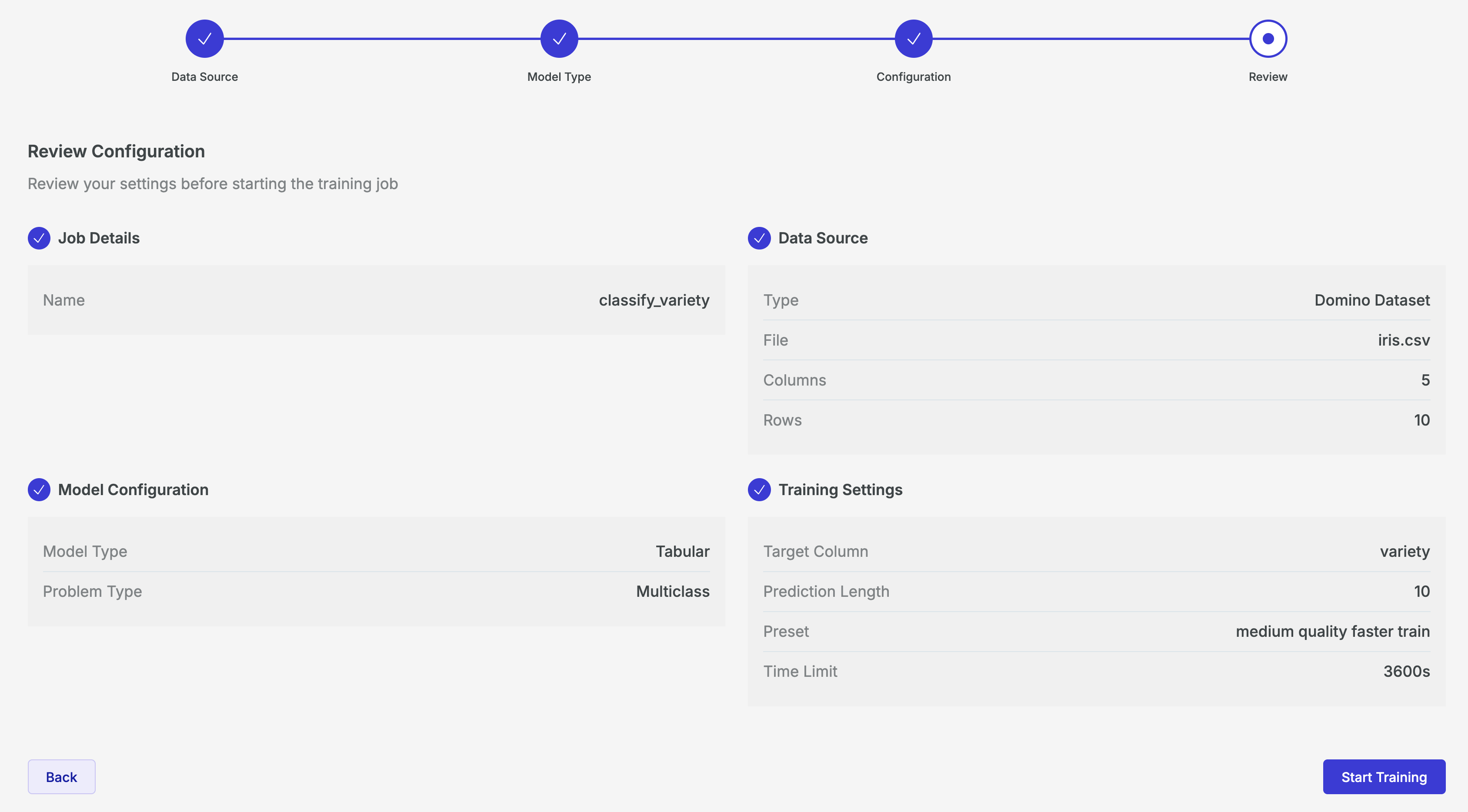
 ### Step 4: Review and launch
Review all your selected settings on the summary screen. If everything looks correct, click **Start Training** to launch the job.
You will be taken to the training run’s overview page where you can monitor progress in real time.
### Step 4: Review and launch
Review all your selected settings on the summary screen. If everything looks correct, click **Start Training** to launch the job.
You will be taken to the training run’s overview page where you can monitor progress in real time.
 ## Training results
Once a training job is launched, its results page provides comprehensive information about the run’s progress and outputs.
The results page is organized into several tabs: **Overview**, **Leaderboard**, **Diagnostics**, **Metrics**, **Outputs**, and **Logs**.
The **Overview** tab displays the training job’s metadata and real-time progress. While the job is running, a progress bar shows the estimated completion percentage and a **Cancel** button is available to stop the run.
The metadata table includes:
| Field | Description |
| ----------------- | ----------------------------------------------------------------- |
| **Run ID** | A unique identifier for this training run. |
| **Model Type** | The predictor type (e.g., `Tabular`). |
| **Problem Type** | The detected or specified problem type (e.g., `Binary`). |
| **Target Column** | The column being predicted (e.g., `Failed`). |
| **Preset** | The quality preset used (e.g., `Medium Quality Faster Train`). |
| **Time Limit** | The configured time limit in seconds (e.g., `3600s`). |
| **Created** | The date and time the job was launched. |
| **Duration** | Total elapsed time for the training run. |
| **Status** | Current status: `Running`, `Completed`, `Failed`, or `Cancelled`. |
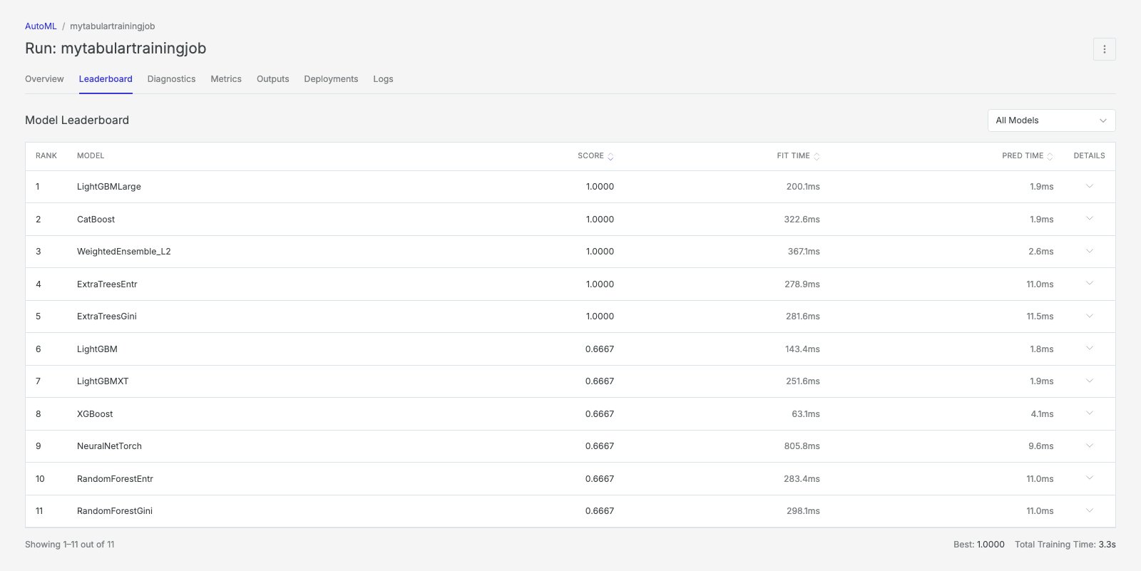
The **Leaderboard** tab ranks all trained models by their validation score. The top-ranked model is the one AutoGluon recommends for deployment.
Models are displayed in a table with the following columns:
| Column | Description |
| ------------- | ------------------------------------------------------------------------------------ |
| **Rank** | Position on the leaderboard (`1` = best). |
| **Model** | Name of the model or ensemble (e.g., `WeightedEnsemble_L2`, `LightGBM`, `CatBoost`). |
| **Score** | Validation score using the selected evaluation metric. |
| **Fit Time** | Time taken to train the model. |
| **Pred Time** | Time taken to generate predictions on the validation set. |
Click the expand arrow next to any model to view additional details:
* **Performance:** Validation score and marginal fit time.
* **Model Info:** Stack level, whether the model can perform inference (`Can Infer`), and other metadata.
Use the **All Models** dropdown to filter the leaderboard by specific model families.
The `WeightedEnsemble` models combine predictions from multiple base models and typically achieve the highest scores. They may have longer prediction times, so consider this trade-off for latency-sensitive applications.
## Training results
Once a training job is launched, its results page provides comprehensive information about the run’s progress and outputs.
The results page is organized into several tabs: **Overview**, **Leaderboard**, **Diagnostics**, **Metrics**, **Outputs**, and **Logs**.
The **Overview** tab displays the training job’s metadata and real-time progress. While the job is running, a progress bar shows the estimated completion percentage and a **Cancel** button is available to stop the run.
The metadata table includes:
| Field | Description |
| ----------------- | ----------------------------------------------------------------- |
| **Run ID** | A unique identifier for this training run. |
| **Model Type** | The predictor type (e.g., `Tabular`). |
| **Problem Type** | The detected or specified problem type (e.g., `Binary`). |
| **Target Column** | The column being predicted (e.g., `Failed`). |
| **Preset** | The quality preset used (e.g., `Medium Quality Faster Train`). |
| **Time Limit** | The configured time limit in seconds (e.g., `3600s`). |
| **Created** | The date and time the job was launched. |
| **Duration** | Total elapsed time for the training run. |
| **Status** | Current status: `Running`, `Completed`, `Failed`, or `Cancelled`. |
The **Leaderboard** tab ranks all trained models by their validation score. The top-ranked model is the one AutoGluon recommends for deployment.
Models are displayed in a table with the following columns:
| Column | Description |
| ------------- | ------------------------------------------------------------------------------------ |
| **Rank** | Position on the leaderboard (`1` = best). |
| **Model** | Name of the model or ensemble (e.g., `WeightedEnsemble_L2`, `LightGBM`, `CatBoost`). |
| **Score** | Validation score using the selected evaluation metric. |
| **Fit Time** | Time taken to train the model. |
| **Pred Time** | Time taken to generate predictions on the validation set. |
Click the expand arrow next to any model to view additional details:
* **Performance:** Validation score and marginal fit time.
* **Model Info:** Stack level, whether the model can perform inference (`Can Infer`), and other metadata.
Use the **All Models** dropdown to filter the leaderboard by specific model families.
The `WeightedEnsemble` models combine predictions from multiple base models and typically achieve the highest scores. They may have longer prediction times, so consider this trade-off for latency-sensitive applications.
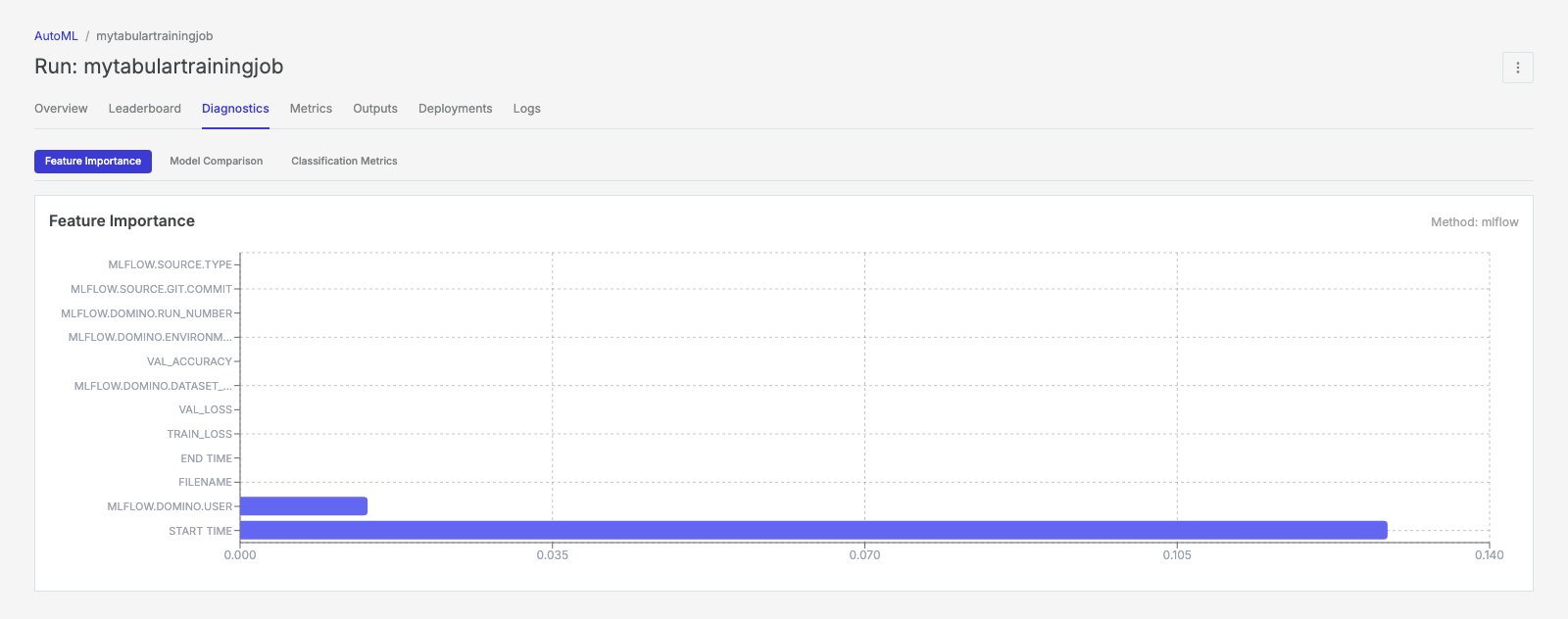
 The **Diagnostics** tab provides visual insights into model behavior. The available sub-tabs depend on the problem type.
**Feature Importance:** A horizontal bar chart ranking features by their contribution to model predictions. Features with the highest importance have the greatest influence on predictions. Use this chart to understand which variables drive your model’s decisions and to identify potential features for engineering or removal.
**Model Comparison:** Side-by-side comparison of all trained models showing model names with color-coded performance bars, validation scores for each model, and a visual comparison helping you understand how different algorithms performed on your data. The best-performing model is highlighted at the top of the comparison.
**Classification Metrics** (binary and multiclass classification only):
This view provides comprehensive classification-specific metrics.
| Component | Description |
| -------------------- | ------------------------------------------------------------------------------------------------------------------------------------------------------------------------------- |
| **Confusion Matrix** | A grid showing predicted vs. actual class labels. Cells are color-coded by frequency, helping identify where the model makes correct predictions and where it confuses classes. |
| **Accuracy** | Overall proportion of correct predictions. |
| **Precision** | Weighted average precision across all classes (proportion of positive predictions that were correct). |
| **Recall** | Weighted average recall across all classes (proportion of actual positives that were correctly identified). |
| **F1-Score** | Weighted average F1-score (harmonic mean of precision and recall). |
| **ROC Curve** | For binary classification only. Plots the true positive rate against the false positive rate at various threshold settings. Includes the AUC (Area Under Curve) score. |
**Regression Diagnostics** (regression only):
This view provides regression-specific metrics and visualizations.
| Component | Description |
| ---------------------------- | -------------------------------------------------------------------------------------------------------------------------------------------------------------------- |
| **R² (R-Squared)** | Coefficient of determination indicating the proportion of variance explained by the model. Values closer to 1.0 indicate better fit. |
| **RMSE** | Root Mean Square Error: average magnitude of prediction errors, in the same units as the target variable. |
| **MAE** | Mean Absolute Error: average absolute difference between predicted and actual values. |
| **MSE** | Mean Square Error: average squared difference between predicted and actual values. |
| **Predicted vs Actual Plot** | Scatter plot comparing predicted values (Y-axis) against actual values (X-axis). Points close to the diagonal line indicate accurate predictions. |
| **Residuals Plot** | Scatter plot showing residuals (prediction errors) against predicted values. Ideally, residuals should be randomly distributed around zero with no visible patterns. |
The **Diagnostics** tab provides visual insights into model behavior. The available sub-tabs depend on the problem type.
**Feature Importance:** A horizontal bar chart ranking features by their contribution to model predictions. Features with the highest importance have the greatest influence on predictions. Use this chart to understand which variables drive your model’s decisions and to identify potential features for engineering or removal.
**Model Comparison:** Side-by-side comparison of all trained models showing model names with color-coded performance bars, validation scores for each model, and a visual comparison helping you understand how different algorithms performed on your data. The best-performing model is highlighted at the top of the comparison.
**Classification Metrics** (binary and multiclass classification only):
This view provides comprehensive classification-specific metrics.
| Component | Description |
| -------------------- | ------------------------------------------------------------------------------------------------------------------------------------------------------------------------------- |
| **Confusion Matrix** | A grid showing predicted vs. actual class labels. Cells are color-coded by frequency, helping identify where the model makes correct predictions and where it confuses classes. |
| **Accuracy** | Overall proportion of correct predictions. |
| **Precision** | Weighted average precision across all classes (proportion of positive predictions that were correct). |
| **Recall** | Weighted average recall across all classes (proportion of actual positives that were correctly identified). |
| **F1-Score** | Weighted average F1-score (harmonic mean of precision and recall). |
| **ROC Curve** | For binary classification only. Plots the true positive rate against the false positive rate at various threshold settings. Includes the AUC (Area Under Curve) score. |
**Regression Diagnostics** (regression only):
This view provides regression-specific metrics and visualizations.
| Component | Description |
| ---------------------------- | -------------------------------------------------------------------------------------------------------------------------------------------------------------------- |
| **R² (R-Squared)** | Coefficient of determination indicating the proportion of variance explained by the model. Values closer to 1.0 indicate better fit. |
| **RMSE** | Root Mean Square Error: average magnitude of prediction errors, in the same units as the target variable. |
| **MAE** | Mean Absolute Error: average absolute difference between predicted and actual values. |
| **MSE** | Mean Square Error: average squared difference between predicted and actual values. |
| **Predicted vs Actual Plot** | Scatter plot comparing predicted values (Y-axis) against actual values (X-axis). Points close to the diagonal line indicate accurate predictions. |
| **Residuals Plot** | Scatter plot showing residuals (prediction errors) against predicted values. Ideally, residuals should be randomly distributed around zero with no visible patterns. |
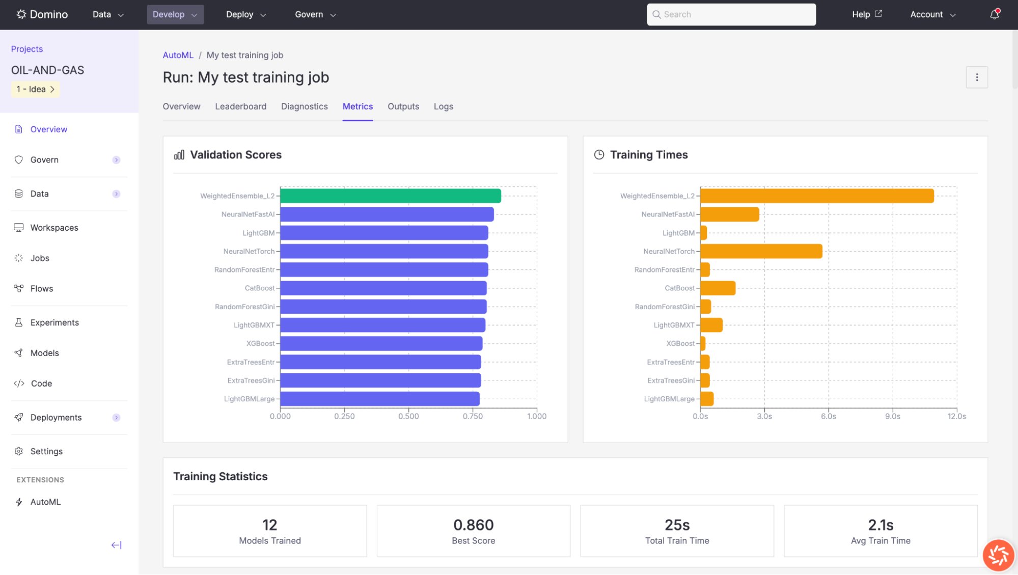
 The **Metrics** tab provides two comparison charts and a summary statistics panel:
**Validation Scores:** A horizontal bar chart comparing every model’s validation score. The best-performing model appears at the top.
**Training Times:** A horizontal bar chart showing how long each model took to train. This helps you evaluate the cost-performance trade-off for each model.
**Training Statistics:** A summary panel displaying key metrics for the overall run.
| Metric | Description |
| -------------------- | ------------------------------------------------------------------------ |
| **Models Trained** | Total number of models trained during the run (e.g., `12`). |
| **Best Score** | The highest validation score achieved across all models (e.g., `0.860`). |
| **Total Train Time** | Total wall-clock time for all model training (e.g., `25s`). |
| **Avg Train Time** | Average training time per model (e.g., `2.1s`). |
The **Metrics** tab provides two comparison charts and a summary statistics panel:
**Validation Scores:** A horizontal bar chart comparing every model’s validation score. The best-performing model appears at the top.
**Training Times:** A horizontal bar chart showing how long each model took to train. This helps you evaluate the cost-performance trade-off for each model.
**Training Statistics:** A summary panel displaying key metrics for the overall run.
| Metric | Description |
| -------------------- | ------------------------------------------------------------------------ |
| **Models Trained** | Total number of models trained during the run (e.g., `12`). |
| **Best Score** | The highest validation score achieved across all models (e.g., `0.860`). |
| **Total Train Time** | Total wall-clock time for all model training (e.g., `25s`). |
| **Avg Train Time** | Average training time per model (e.g., `2.1s`). |
 The **Outputs** tab provides two ways to export your trained model:
**Deployment Package:** A complete, self-contained package with everything needed to deploy the model as an API endpoint. You specify an output directory (default: `/domino/datasets/local//`) and optionally enable **Optimize for Inference**. Click **Create Package** to generate the deployment artifacts.
The deployment package contains:
| File | Description |
| -------------------- | ----------------------------------------------------------------------- |
| **model/** | Trained model artifacts generated by AutoGluon. |
| **inference.py** | A Python inference script that loads the model and returns predictions. |
| **requirements.txt** | Python dependencies needed to run inference. |
| **Dockerfile** | A container configuration file for building a deployment image. |
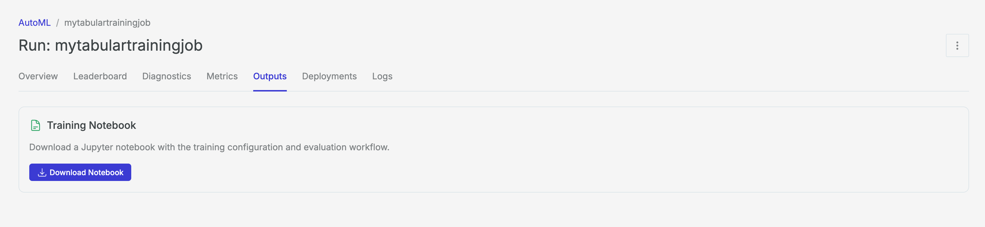
**Training Notebook:** Click **Download Notebook** to get a Jupyter notebook with the full training configuration, evaluation code, and deployment instructions. This notebook serves as a reproducible record of the experiment and a starting point for further customization.
The **Outputs** tab provides two ways to export your trained model:
**Deployment Package:** A complete, self-contained package with everything needed to deploy the model as an API endpoint. You specify an output directory (default: `/domino/datasets/local//`) and optionally enable **Optimize for Inference**. Click **Create Package** to generate the deployment artifacts.
The deployment package contains:
| File | Description |
| -------------------- | ----------------------------------------------------------------------- |
| **model/** | Trained model artifacts generated by AutoGluon. |
| **inference.py** | A Python inference script that loads the model and returns predictions. |
| **requirements.txt** | Python dependencies needed to run inference. |
| **Dockerfile** | A container configuration file for building a deployment image. |
**Training Notebook:** Click **Download Notebook** to get a Jupyter notebook with the full training configuration, evaluation code, and deployment instructions. This notebook serves as a reproducible record of the experiment and a starting point for further customization.
 The **Logs** tab displays the real-time console output from the AutoGluon training process.
This includes detailed information about each model being trained, hyperparameters used, validation results, and any warnings or errors.
Logs are useful for debugging failed runs and understanding the training process in detail.
The **Forecast** tab is available only for completed Time Series training jobs. It allows you to generate future predictions using your trained model.
**Job Information**
Displays key configuration details from training:
* **Target Column:** The variable being forecasted.
* **Time Column:** The timestamp/date column used for time ordering.
* **ID Column:** The identifier column for multi-series forecasting (if configured).
**Generating a Forecast**
1. Set **Prediction Horizon**: Enter the number of future time steps to predict (1-365). This defaults to the prediction length specified during training.
2. Click **Generate Forecast**: The model produces predictions for the specified number of time steps into the future.
**Forecast Results**
After generation, results are displayed in a table format showing:
| Column | Description |
| ------------------------ | ---------------------------------------------------------------------------------------------- |
| **Time Step** | The future time period index (1, 2, 3, etc.). |
| **Predicted Value** | The forecasted value for each time step. |
| **Confidence Intervals** | Lower and upper bounds at various quantiles (if available), indicating prediction uncertainty. |
For multi-series forecasting (when an ID column was specified), predictions are grouped by series identifier.
## Deploy a model
After training is complete, you can deploy the best model directly from the AutoML interface.
### Export a Deployment Package
1. Navigate to the **Outputs** tab of your completed training run.
2. Verify the output directory path under **Deployment Package**.
3. (Optional) Check **Optimize for inference** to reduce model size and improve prediction latency.
4. Click **Create Package**.
The generated package is saved to the specified directory in your Domino project’s dataset storage. It includes the model artifacts, inference script, requirements file, and Dockerfile.
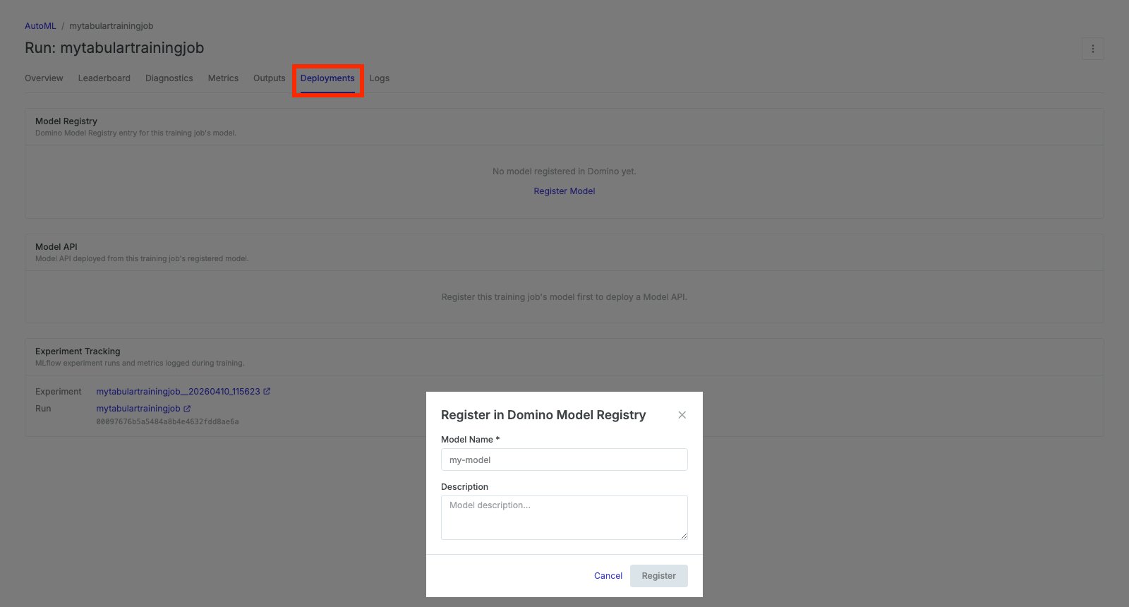
### Register a Model
To register your model in Domino’s Model Registry for versioning, governance, and deployment:
1. Click the **Register** button in the top-right corner of the training results page.
2. In the **Deploy to Model Registry** dialog, enter a **Model Name**.
3. Select the **Model Type** (e.g., `Tabular`).
4. Optionally add a description to document the model’s purpose and training context.
5. Click **Register** to save the model to the registry.
Once registered, the model appears in the **Models** section of your Domino project and can be deployed as an API endpoint, used in batch scoring, or shared across teams.
The **Logs** tab displays the real-time console output from the AutoGluon training process.
This includes detailed information about each model being trained, hyperparameters used, validation results, and any warnings or errors.
Logs are useful for debugging failed runs and understanding the training process in detail.
The **Forecast** tab is available only for completed Time Series training jobs. It allows you to generate future predictions using your trained model.
**Job Information**
Displays key configuration details from training:
* **Target Column:** The variable being forecasted.
* **Time Column:** The timestamp/date column used for time ordering.
* **ID Column:** The identifier column for multi-series forecasting (if configured).
**Generating a Forecast**
1. Set **Prediction Horizon**: Enter the number of future time steps to predict (1-365). This defaults to the prediction length specified during training.
2. Click **Generate Forecast**: The model produces predictions for the specified number of time steps into the future.
**Forecast Results**
After generation, results are displayed in a table format showing:
| Column | Description |
| ------------------------ | ---------------------------------------------------------------------------------------------- |
| **Time Step** | The future time period index (1, 2, 3, etc.). |
| **Predicted Value** | The forecasted value for each time step. |
| **Confidence Intervals** | Lower and upper bounds at various quantiles (if available), indicating prediction uncertainty. |
For multi-series forecasting (when an ID column was specified), predictions are grouped by series identifier.
## Deploy a model
After training is complete, you can deploy the best model directly from the AutoML interface.
### Export a Deployment Package
1. Navigate to the **Outputs** tab of your completed training run.
2. Verify the output directory path under **Deployment Package**.
3. (Optional) Check **Optimize for inference** to reduce model size and improve prediction latency.
4. Click **Create Package**.
The generated package is saved to the specified directory in your Domino project’s dataset storage. It includes the model artifacts, inference script, requirements file, and Dockerfile.
### Register a Model
To register your model in Domino’s Model Registry for versioning, governance, and deployment:
1. Click the **Register** button in the top-right corner of the training results page.
2. In the **Deploy to Model Registry** dialog, enter a **Model Name**.
3. Select the **Model Type** (e.g., `Tabular`).
4. Optionally add a description to document the model’s purpose and training context.
5. Click **Register** to save the model to the registry.
Once registered, the model appears in the **Models** section of your Domino project and can be deployed as an API endpoint, used in batch scoring, or shared across teams.
 ## Best practices
* **Review data quality before training.** Use the Data Exploration tool to inspect missing values, outliers, and column types. Address high-priority recommendations (especially dropping or imputing columns with more than 30% missing data) before starting a training job.
* **Choose the right preset.** The Medium Quality (Faster) preset is a good starting point for rapid iteration. Once you have identified a promising dataset and target, switch to Best Quality for production models, especially on smaller datasets where the additional training time yields meaningful improvements.
* **Set an appropriate time limit.** A longer time limit allows AutoGluon to train more models and explore more hyperparameter configurations. For initial exploration, 600–1800 seconds is often sufficient. For production runs, consider 3600 seconds or more.
* **Exclude identifier columns.** Columns with all unique values (flagged as identifiers) do not contribute meaningful signal and should be dropped before training. AutoML will flag these in both Column Analysis and Recommended Transformations.
* **Examine feature importance.** After training, review the Feature Importance chart on the Diagnostics tab. If unimportant features dominate, consider removing them and retraining to reduce noise and improve generalization.
* **Consider the prediction time trade-off.** Ensemble models (e.g., WeightedEnsemble\_L2) typically achieve the best validation scores but may have higher inference latency. For real-time applications, compare leaderboard scores with prediction times and consider selecting a simpler model that meets your latency requirements. Use the exported notebook for reproducibility. Download the Training Notebook from the Outputs tab to preserve a complete record of your training configuration. This notebook can be re-run in a Domino Workspace and serves as the starting point for any custom modifications.
## Best practices
* **Review data quality before training.** Use the Data Exploration tool to inspect missing values, outliers, and column types. Address high-priority recommendations (especially dropping or imputing columns with more than 30% missing data) before starting a training job.
* **Choose the right preset.** The Medium Quality (Faster) preset is a good starting point for rapid iteration. Once you have identified a promising dataset and target, switch to Best Quality for production models, especially on smaller datasets where the additional training time yields meaningful improvements.
* **Set an appropriate time limit.** A longer time limit allows AutoGluon to train more models and explore more hyperparameter configurations. For initial exploration, 600–1800 seconds is often sufficient. For production runs, consider 3600 seconds or more.
* **Exclude identifier columns.** Columns with all unique values (flagged as identifiers) do not contribute meaningful signal and should be dropped before training. AutoML will flag these in both Column Analysis and Recommended Transformations.
* **Examine feature importance.** After training, review the Feature Importance chart on the Diagnostics tab. If unimportant features dominate, consider removing them and retraining to reduce noise and improve generalization.
* **Consider the prediction time trade-off.** Ensemble models (e.g., WeightedEnsemble\_L2) typically achieve the best validation scores but may have higher inference latency. For real-time applications, compare leaderboard scores with prediction times and consider selecting a simpler model that meets your latency requirements. Use the exported notebook for reproducibility. Download the Training Notebook from the Outputs tab to preserve a complete record of your training configuration. This notebook can be re-run in a Domino Workspace and serves as the starting point for any custom modifications.