> ## Documentation Index
> Fetch the complete documentation index at: https://docs.domino.ai/llms.txt
> Use this file to discover all available pages before exploring further.
# Develop your MATLAB model
When you are developing your model, you can use Workspaces to quickly execute code, see outputs, and make iterative improvements.
You previously learned [how to start a Workspace](/cloud/getting-started/for-modelers-and-builders/get-started-matlab/4-start-workspace) and explored basic options.
In this topic, you will use your workspace to load, explore, and transform data. After the data has been prepared, you will train a model.
## Step 1: Load and explore the dataset
1. Click the browser tab to return to the Workspace.
2. Click **New** > **Live Script** to create a MATLAB Live Script.
3. Go to **Save > Save As…** to save it as `ber_hot_weather.mlx`.
4. Copy and paste the following command:
```matlab theme={null}
opts = detectImportOptions('tegel.csv');
```
5. Click **Run**.
6. Copy and paste the following commands to load `tegel.csv` into MATLAB. Then, click **Run**. This loads the data using the `readtable()` function, giving it the import options object as a second argument.
```matlab theme={null}
opts.SelectedVariableNames = {'DATE', 'PRCP', 'TMIN', 'TMAX'};
opts = setvartype(opts, {'DATE','PRCP','TMIN','TMAX'},{'datetime','double', 'double', 'double'});
berWeatherTbl = readtable("tegel.csv", opts);
head(berWeatherTbl)
```
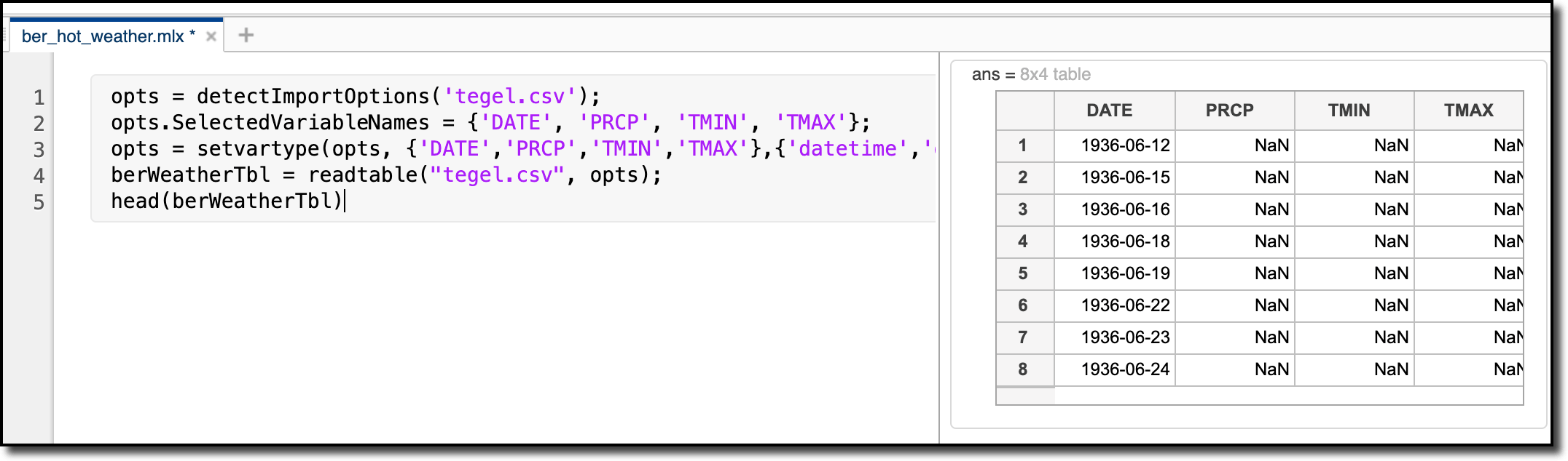
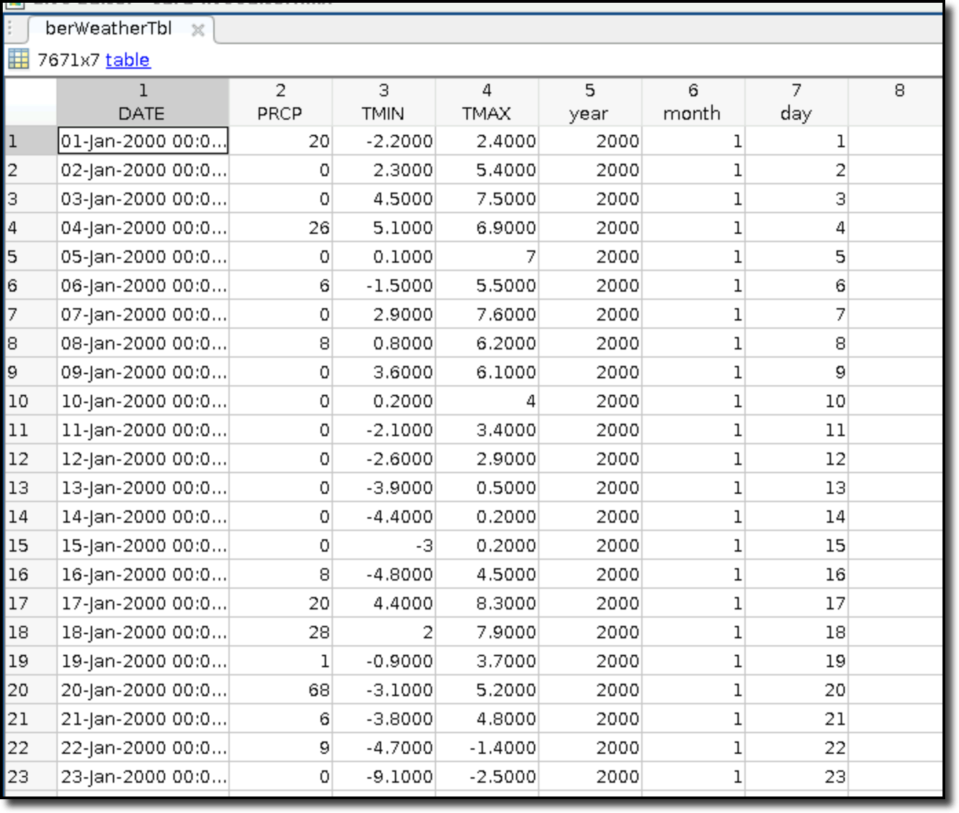
These commands loaded the following columns and assigned data types to them.
* **Date** – date the temperature was read
* **PRCP** – total precipitation for the day
* **TMIN** – lowest temperature measured that day
* **TMAX** – highest temperature measured that day
The result will look similar to the following:
 7. Click **Section Break** to create a new section in your script.
Your cursor must be at the end of the previous section. You might have to go to the Insert tab to find **Section Break**.
1. Copy and paste the following command to format the dates into a Year/Month/Day format and store each field as a table variable. This helps you examine the data.
```matlab theme={null}
[berWeatherTbl.year, berWeatherTbl.month, berWeatherTbl.day] = ymd(berWeatherTbl.DATE);
```
2. Copy and paste the following command to limit the dataset to temperatures between January 2000 and December 2019, inclusive, by removing rows with data outside this range. This speeds data processing.
```matlab theme={null}
berWeatherTbl = berWeatherTbl(berWeatherTbl.year > 1999 & berWeatherTbl.year < max(berWeatherTbl.year) , :);
```
3. Copy and paste the following commands to divide all temperature data by 10 to get the temperatures in full Celsius degrees. You might have noticed that temperatures in the **TMAX** or **TMIN** columns look a bit odd. This is because NOAA uses a temperature format consisting of a tenth-of-a-degree in the Celsius scale.
```matlab theme={null}
berWeatherTbl.TMAX = berWeatherTbl.TMAX/10;
berWeatherTbl.TMIN = berWeatherTbl.TMIN/10;
```
4. Copy and paste the following command to complete missing data with interpolated information.
```matlab theme={null}
berWeatherTbl = fillmissing(berWeatherTbl, 'linear');
```
5. Copy and paste the following `head()` function to preview the start of the table.
```matlab theme={null}
head(berWeatherTbl)
```
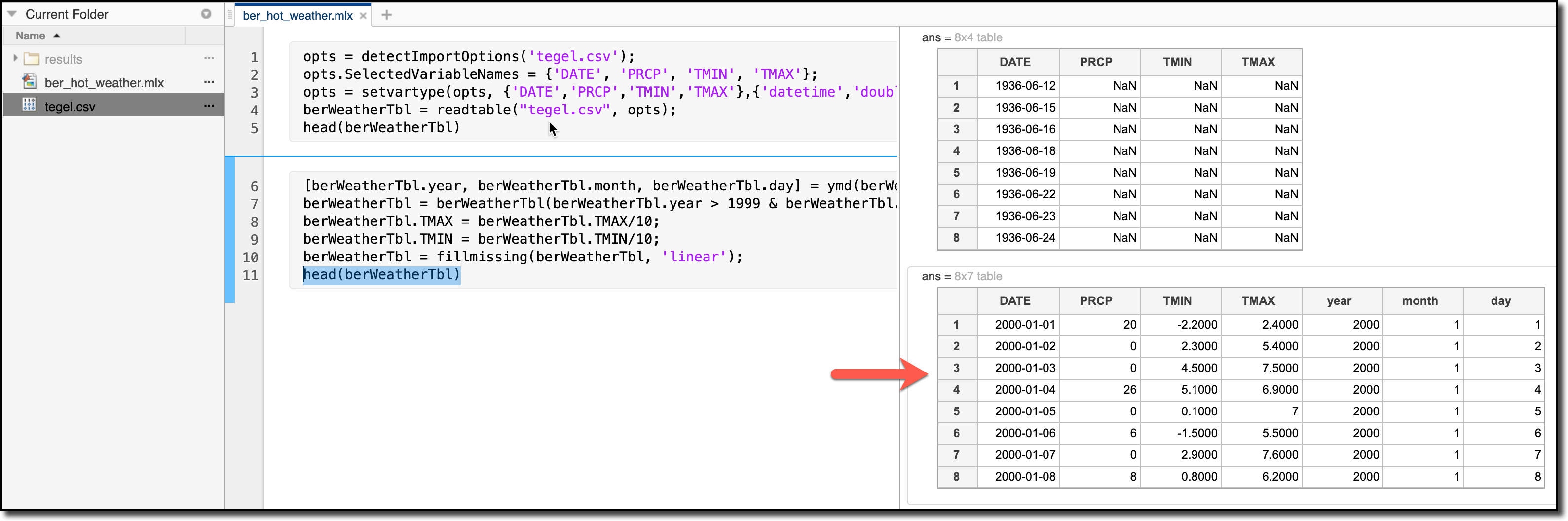
6. Click **Run**. The result looks like the following:
7. Click **Section Break** to create a new section in your script.
Your cursor must be at the end of the previous section. You might have to go to the Insert tab to find **Section Break**.
1. Copy and paste the following command to format the dates into a Year/Month/Day format and store each field as a table variable. This helps you examine the data.
```matlab theme={null}
[berWeatherTbl.year, berWeatherTbl.month, berWeatherTbl.day] = ymd(berWeatherTbl.DATE);
```
2. Copy and paste the following command to limit the dataset to temperatures between January 2000 and December 2019, inclusive, by removing rows with data outside this range. This speeds data processing.
```matlab theme={null}
berWeatherTbl = berWeatherTbl(berWeatherTbl.year > 1999 & berWeatherTbl.year < max(berWeatherTbl.year) , :);
```
3. Copy and paste the following commands to divide all temperature data by 10 to get the temperatures in full Celsius degrees. You might have noticed that temperatures in the **TMAX** or **TMIN** columns look a bit odd. This is because NOAA uses a temperature format consisting of a tenth-of-a-degree in the Celsius scale.
```matlab theme={null}
berWeatherTbl.TMAX = berWeatherTbl.TMAX/10;
berWeatherTbl.TMIN = berWeatherTbl.TMIN/10;
```
4. Copy and paste the following command to complete missing data with interpolated information.
```matlab theme={null}
berWeatherTbl = fillmissing(berWeatherTbl, 'linear');
```
5. Copy and paste the following `head()` function to preview the start of the table.
```matlab theme={null}
head(berWeatherTbl)
```
6. Click **Run**. The result looks like the following:
 Click **Save** occasionally to save your script.
8. Click **Section Break** to create another section in your Live Script. In this section, you’ll calculate how many hot days have occurred in Berlin since the year 2000. To calculate this, copy and paste the following command to define a hot day as 29 degrees Celsius for the baseline threshold.
```matlab theme={null}
hotDayThreshold = 29;
```
9. Copy and paste the following command to calculate how many hot days have occurred since (and including) the year 2000. This command creates a table column indexing the days with maximum temperatures (**TMAX**) that meet or exceed the hot day threshold.
```matlab theme={null}
berWeatherTbl.HotDayFlag = berWeatherTbl.TMAX >= hotDayThreshold;
```
1. Copy and paste the following command to use `groupsummary()` to count how many hot days were flagged:
```matlab theme={null}
numHotDaysPerYear = groupsummary(berWeatherTbl, 'year', 'sum', 'HotDayFlag');
```
2. Copy and paste the following command to repeat the same approach to find the highest temperature of each year:
```matlab theme={null}
maxTempOfYear = groupsummary(berWeatherTbl, 'year', 'max', 'TMAX');
```
3. Copy and paste the following command to combine the variables to create a table named `annualMaxTbl`:
```matlab theme={null}
annualMaxTbl = join(numHotDaysPerYear, maxTempOfYear);
annualMaxTbl.Properties.VariableNames = {'Year', 'daysInYear', 'hotDayCount', 'maxTemp'};
annualMaxTbl
```
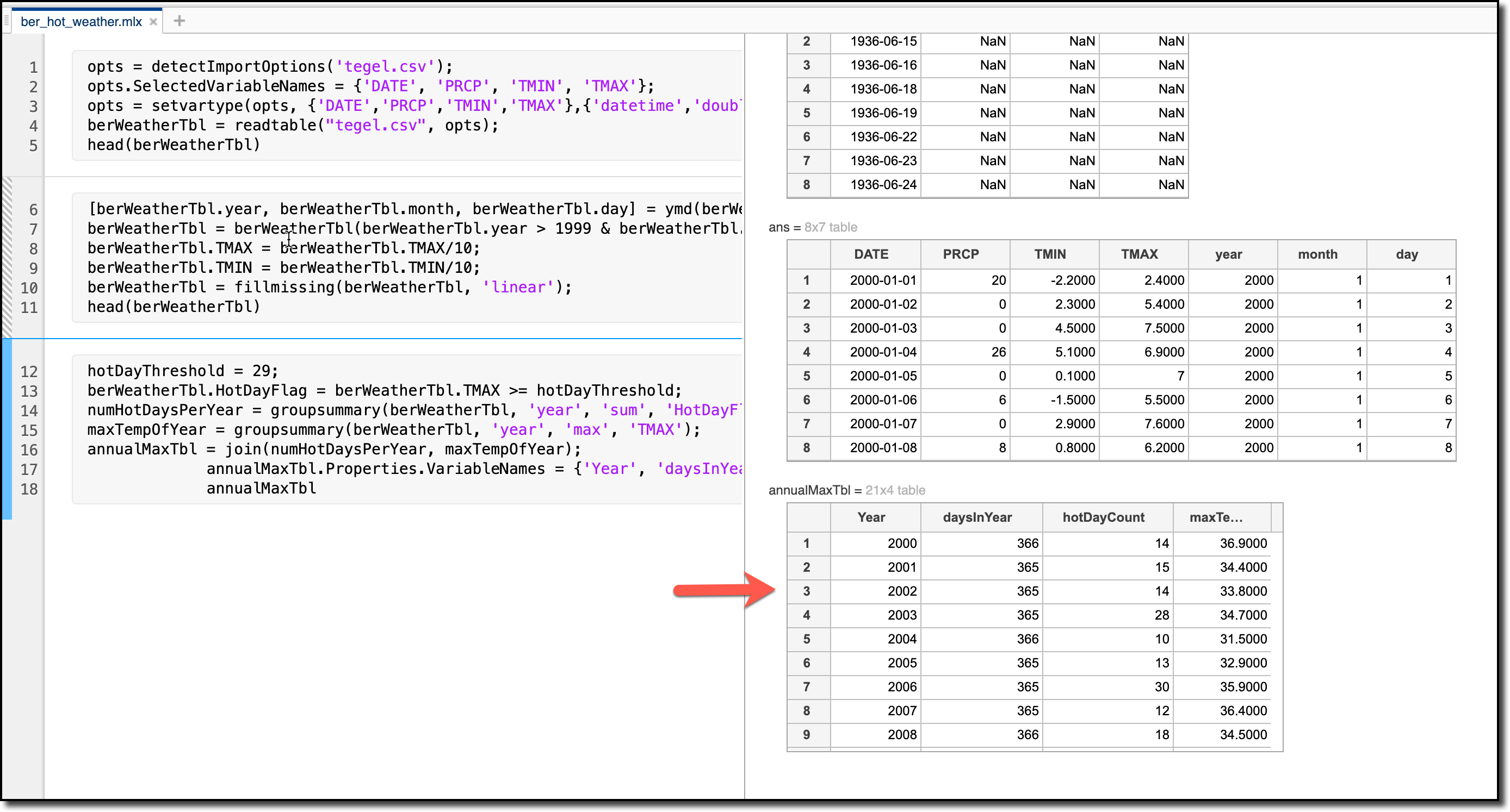
4. Click **Run Section**. The table looks like the following:
Click **Save** occasionally to save your script.
8. Click **Section Break** to create another section in your Live Script. In this section, you’ll calculate how many hot days have occurred in Berlin since the year 2000. To calculate this, copy and paste the following command to define a hot day as 29 degrees Celsius for the baseline threshold.
```matlab theme={null}
hotDayThreshold = 29;
```
9. Copy and paste the following command to calculate how many hot days have occurred since (and including) the year 2000. This command creates a table column indexing the days with maximum temperatures (**TMAX**) that meet or exceed the hot day threshold.
```matlab theme={null}
berWeatherTbl.HotDayFlag = berWeatherTbl.TMAX >= hotDayThreshold;
```
1. Copy and paste the following command to use `groupsummary()` to count how many hot days were flagged:
```matlab theme={null}
numHotDaysPerYear = groupsummary(berWeatherTbl, 'year', 'sum', 'HotDayFlag');
```
2. Copy and paste the following command to repeat the same approach to find the highest temperature of each year:
```matlab theme={null}
maxTempOfYear = groupsummary(berWeatherTbl, 'year', 'max', 'TMAX');
```
3. Copy and paste the following command to combine the variables to create a table named `annualMaxTbl`:
```matlab theme={null}
annualMaxTbl = join(numHotDaysPerYear, maxTempOfYear);
annualMaxTbl.Properties.VariableNames = {'Year', 'daysInYear', 'hotDayCount', 'maxTemp'};
annualMaxTbl
```
4. Click **Run Section**. The table looks like the following:
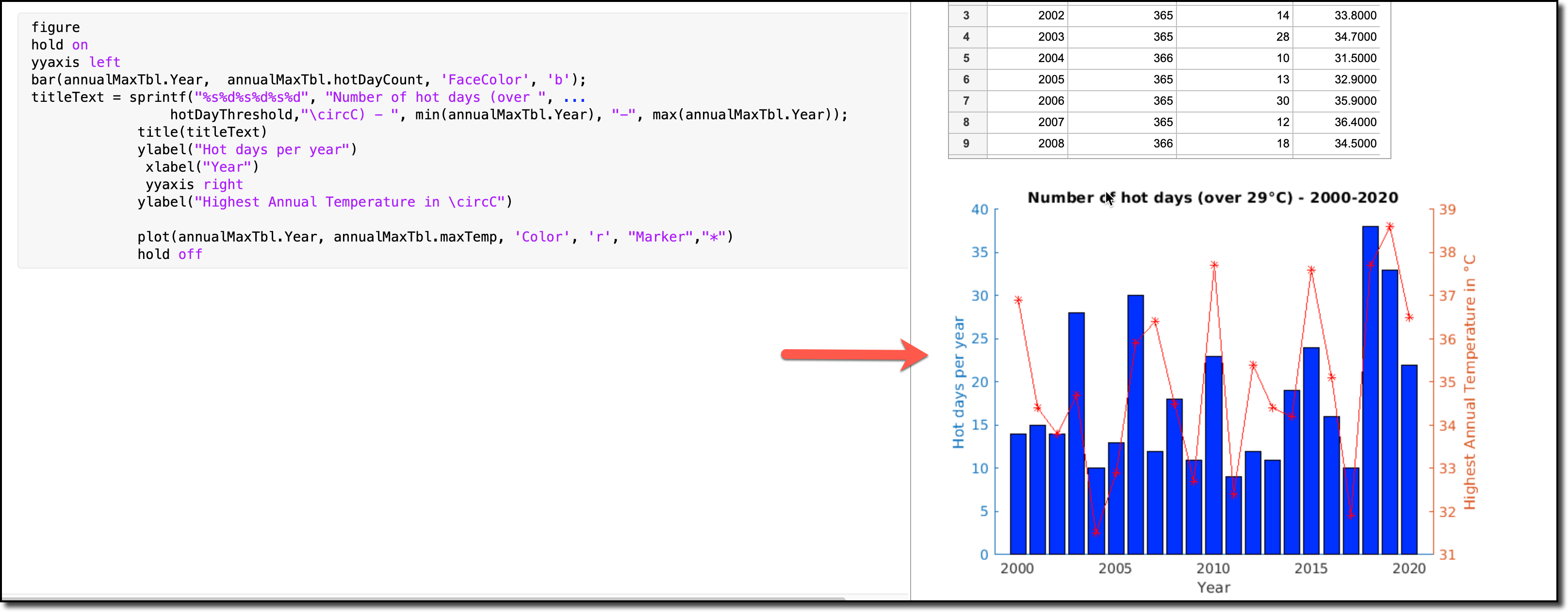
 10. Click **Section Break** to create another section in your Live Script. In this section, you’ll visualize the weather data using a chart with that combines a bar graph and line graph. The chart will use two y-axes.
The bar graph will represent the hot day count (for a given year), and the line graph will represent the highest annual temperature (in Celsius, for a given year). The y-axis on the left side of the chart will correspond to the hot day count, and the y-axis on the right side of the chart will correspond to the highest annual temperature.
* Copy and paste the following to create a hot day count bar graph.
```matlab theme={null}
figure
hold on
yyaxis left
bar(annualMaxTbl.Year, annualMaxTbl.hotDayCount, 'FaceColor', 'b');
```
* Copy and paste the following to add a title and labels to the x-axis and left side y-axis.
```matlab theme={null}
titleText = sprintf("%s%d%s%d%s%d", "Number of hot days (over ", hotDayThreshold,"\circC) - ", min(annualMaxTbl.Year), "-", max(annualMaxTbl.Year));
title(titleText)
ylabel("Hot days per year")
xlabel("Year")
```
* Copy and paste the following to draw the line plot for the highest temperature each year.
```matlab theme={null}
yyaxis right
ylabel("Highest Annual Temperature in \circC")
plot(annualMaxTbl.Year, annualMaxTbl.maxTemp, 'Color', 'r', "Marker","*")
hold off
```
* Click **Run Section**. Your chart should look something like the following:
10. Click **Section Break** to create another section in your Live Script. In this section, you’ll visualize the weather data using a chart with that combines a bar graph and line graph. The chart will use two y-axes.
The bar graph will represent the hot day count (for a given year), and the line graph will represent the highest annual temperature (in Celsius, for a given year). The y-axis on the left side of the chart will correspond to the hot day count, and the y-axis on the right side of the chart will correspond to the highest annual temperature.
* Copy and paste the following to create a hot day count bar graph.
```matlab theme={null}
figure
hold on
yyaxis left
bar(annualMaxTbl.Year, annualMaxTbl.hotDayCount, 'FaceColor', 'b');
```
* Copy and paste the following to add a title and labels to the x-axis and left side y-axis.
```matlab theme={null}
titleText = sprintf("%s%d%s%d%s%d", "Number of hot days (over ", hotDayThreshold,"\circC) - ", min(annualMaxTbl.Year), "-", max(annualMaxTbl.Year));
title(titleText)
ylabel("Hot days per year")
xlabel("Year")
```
* Copy and paste the following to draw the line plot for the highest temperature each year.
```matlab theme={null}
yyaxis right
ylabel("Highest Annual Temperature in \circC")
plot(annualMaxTbl.Year, annualMaxTbl.maxTemp, 'Color', 'r', "Marker","*")
hold off
```
* Click **Run Section**. Your chart should look something like the following:
 ## Step 2: MATLAB - Generate predictions from data
In this section, you will use an interactive machine-learning MATLAB application called **Regression Learner** to develop a model that can predict the weather for the next 20 days.
### 1: Partition the data
You must partition the data that will be used with Regression Learner into the following sets:
* Data to train the model
* Data to test the model
1. Click **Section Break** in the Live Script and copy and paste the following code to remove the `HotDayFlag` column.
```matlab theme={null}
berWeatherTbl.HotDayFlag = [];
```
2. Copy and paste the following to partition the data.
```matlab theme={null}
cv = cvpartition(berWeatherTbl.year, 'Holdout', 0.3);
dataTrain = berWeatherTbl(cv.training, :);
dataTest = berWeatherTbl(cv.test, :);
```
3. Click **Run Section**.
### 2: Train the model
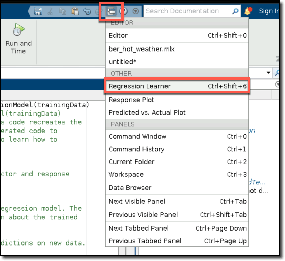
1. Click the **APPS** tab and click Regression Learner app. If you do not see the Regression Learner app, click the arrow to expand the full app list.
## Step 2: MATLAB - Generate predictions from data
In this section, you will use an interactive machine-learning MATLAB application called **Regression Learner** to develop a model that can predict the weather for the next 20 days.
### 1: Partition the data
You must partition the data that will be used with Regression Learner into the following sets:
* Data to train the model
* Data to test the model
1. Click **Section Break** in the Live Script and copy and paste the following code to remove the `HotDayFlag` column.
```matlab theme={null}
berWeatherTbl.HotDayFlag = [];
```
2. Copy and paste the following to partition the data.
```matlab theme={null}
cv = cvpartition(berWeatherTbl.year, 'Holdout', 0.3);
dataTrain = berWeatherTbl(cv.training, :);
dataTest = berWeatherTbl(cv.test, :);
```
3. Click **Run Section**.
### 2: Train the model
1. Click the **APPS** tab and click Regression Learner app. If you do not see the Regression Learner app, click the arrow to expand the full app list.
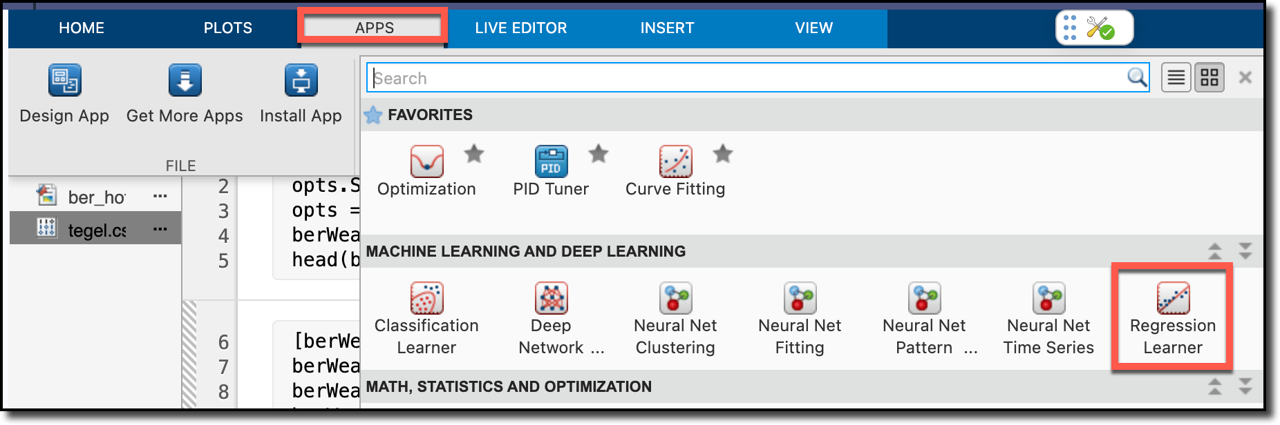 If Regression Learner is not in the apps list, contact your IT team or your MathWorks account manager for assistance.
The application opens in a new window.
2. Click **New Session** and select **From Workspace**.
3. Use the New Session window to specify the input variables for predictions in your model, as well as the outputs (or responses) you want to predict. In this tutorial, the output is the maximum temperature.
1. For the input variable, from the **Workspace Variable** list, select **dataTrain**.
2. For the output, in the Response section, select **TMAX** (maximum temperature).
3. Select **PRCP**, **TMIN**, **year**, **month**, and **day** in the Predictors section.
If Regression Learner is not in the apps list, contact your IT team or your MathWorks account manager for assistance.
The application opens in a new window.
2. Click **New Session** and select **From Workspace**.
3. Use the New Session window to specify the input variables for predictions in your model, as well as the outputs (or responses) you want to predict. In this tutorial, the output is the maximum temperature.
1. For the input variable, from the **Workspace Variable** list, select **dataTrain**.
2. For the output, in the Response section, select **TMAX** (maximum temperature).
3. Select **PRCP**, **TMIN**, **year**, **month**, and **day** in the Predictors section.
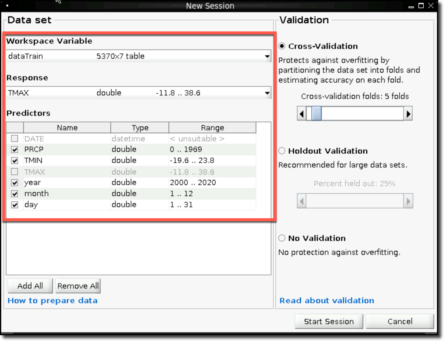 4. Click **Start Session**. The Regression Learner window refreshes and shows the original data set and the values of **TMAX**.
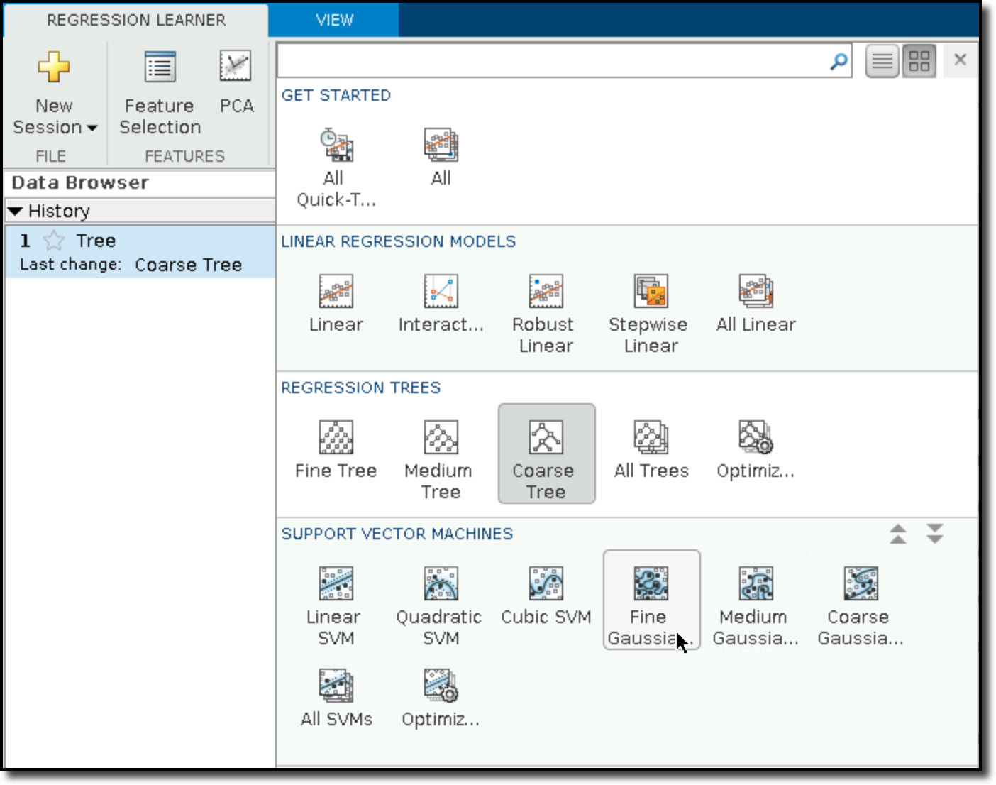
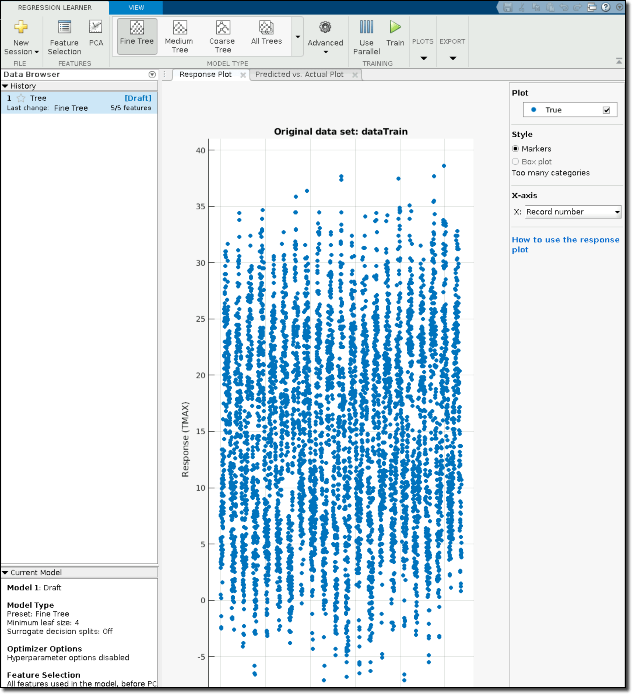 4. Select the type of model to be used for model training. For this tutorial, select **Coarse Tree**.
1. Regression Learner runs best on a container with multiple cores because it can run in parallel and produce models rapidly. If you are using a single-core container, click **Use Parallel** in Regression Learner to turn off parallel processing.
2. Click **Train** to start the model training process. The Domino container spins up a *parallel pool* which is a method to optimize the model training.
5. Select **Fine Gaussian SVM** to compare the results to **Coarse Tree**. You can select additional models or even select all models and compare the results to identify the best fit for your data.
1. Click the arrow to access the model types.
4. Select the type of model to be used for model training. For this tutorial, select **Coarse Tree**.
1. Regression Learner runs best on a container with multiple cores because it can run in parallel and produce models rapidly. If you are using a single-core container, click **Use Parallel** in Regression Learner to turn off parallel processing.
2. Click **Train** to start the model training process. The Domino container spins up a *parallel pool* which is a method to optimize the model training.
5. Select **Fine Gaussian SVM** to compare the results to **Coarse Tree**. You can select additional models or even select all models and compare the results to identify the best fit for your data.
1. Click the arrow to access the model types.
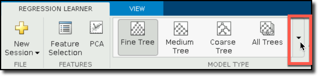
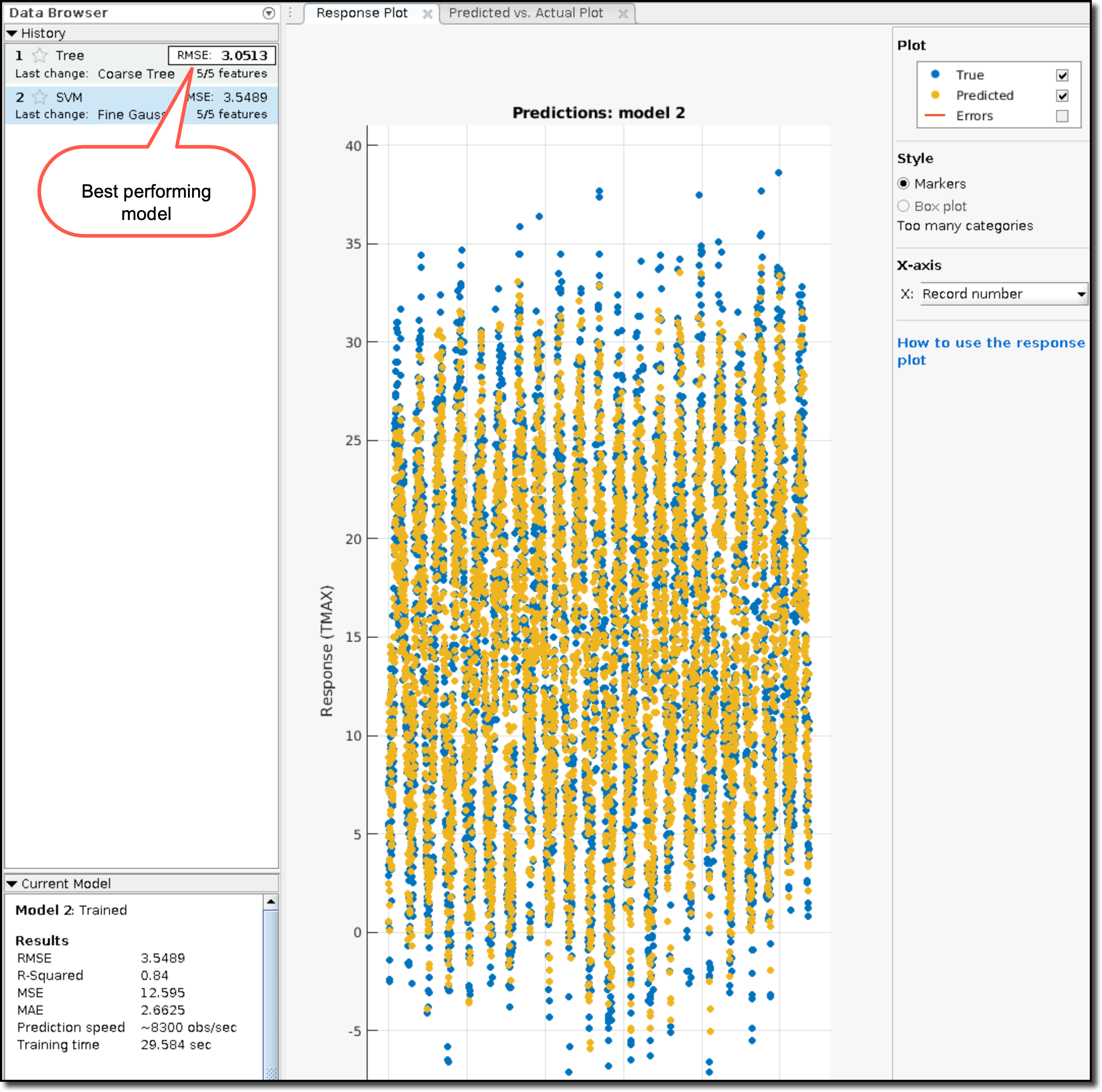
 2. Click **Train**. The model list automatically selects the model that best fits the data. Several visualizations are shown to demonstrate this.
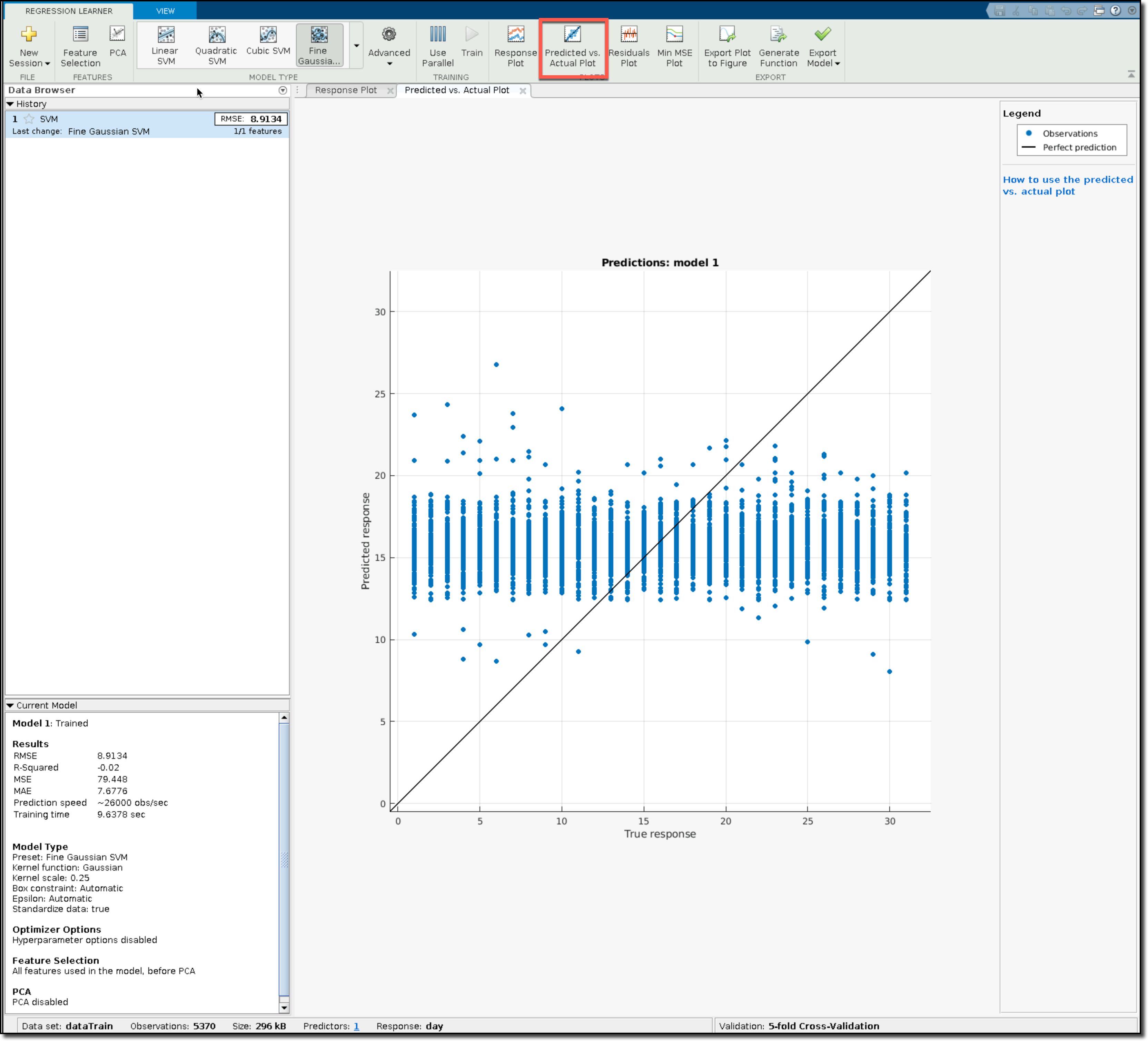
 3. Click **Predicted vs. Actual Plot** open a chart that shows how many predictions the model made that fit correct values in the data. The closer the predictions are to the diagonal, the better the predictions.
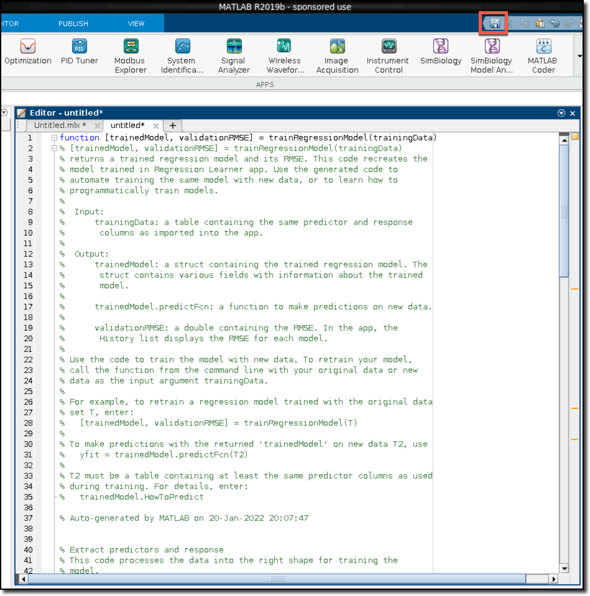
 6. Click **Generate Function** to use Regression Learner to create a function that will be used to deploy the model with Domino. MATLAB generates the function in an M-file. Click **Save** to save the file as `trainRegressionModel.m`.
 ### 3: Export the model
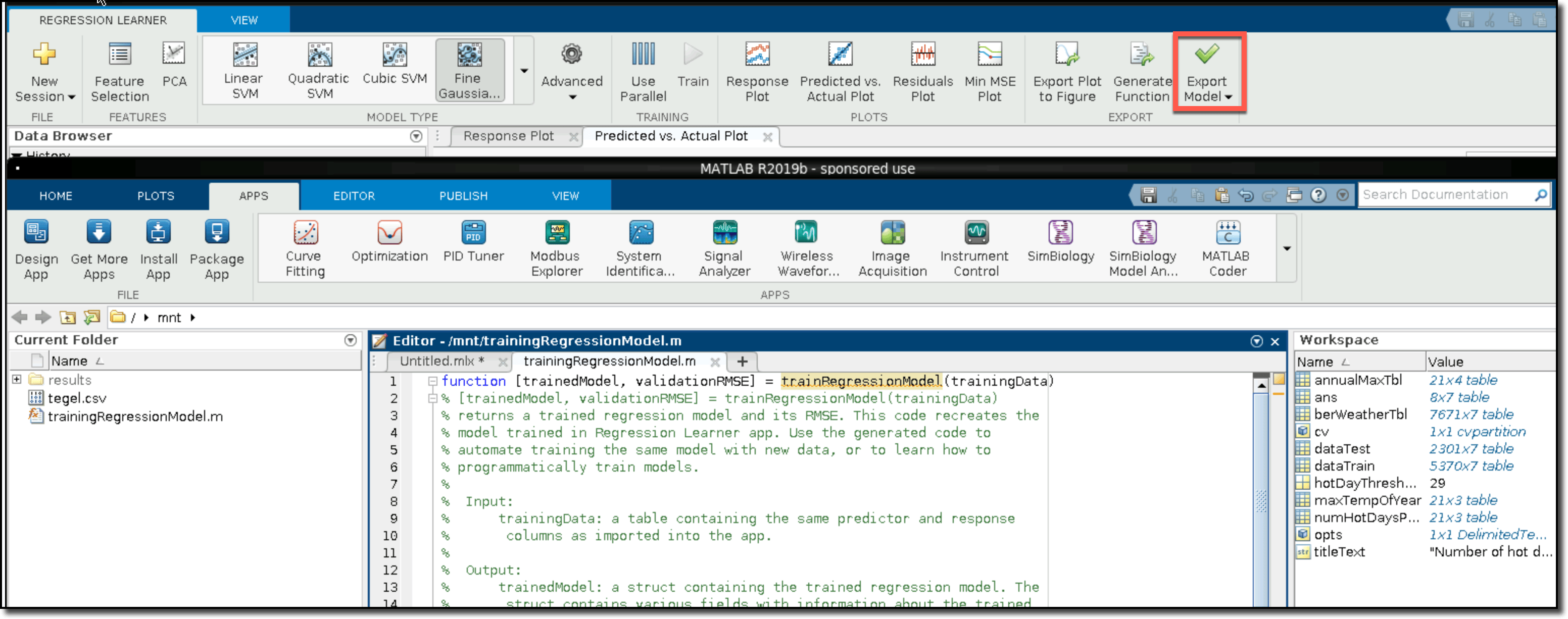
1. Click **Export Model** to export the model to your Domino workspace so you can use it for predictions.
If you cannot find the **Export** button, you might have to switch back to the Regression Learner. See the following images for guidance.
### 3: Export the model
1. Click **Export Model** to export the model to your Domino workspace so you can use it for predictions.
If you cannot find the **Export** button, you might have to switch back to the Regression Learner. See the following images for guidance.
 2. Type a name for the model, such as **weatherModel**, and click **OK**.
3. Close the Regression Learner app and you can see the trained model in your workspace.
2. Type a name for the model, such as **weatherModel**, and click **OK**.
3. Close the Regression Learner app and you can see the trained model in your workspace.
 Notice that the Command Window shows information about how to use the model to make predictions with the following line of code:
```matlab theme={null}
yFit = weatherModel.predictFcn(T);
```
If you input a table of data, this line of code will output a prediction (as a table). The input table must include data organized like the data you used in `berWeatherTbl` – date, precipitation, minimum temperature, month, day and year. It must not include **TMAX**, as that value will be predicted. The model will predict the **TMAX** value and include it in `yFit`.
### 4: Test the model
1. To test the model with the data you partitioned earlier, create a **Section Break** in your Live Script (`ber_hot_weather.mlx`). Copy and paste the following to use the model with the test data and the function call that was listed in the Command Window.
```matlab theme={null}
yFit = weatherModel.predictFcn(dataTest);
```
2. Copy and paste the following to compare the results column to the actual values in the test data set.
```matlab theme={null}
err = yFit - dataTest.TMAX;
```
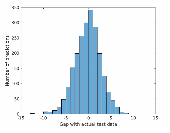
3. Copy and paste the following to draw a histogram to visualize the results.
```matlab theme={null}
figure;
histogram(err)
xlim([-15 15])
ylabel('Number of predictions');
xlabel('Gap with actual test data')
```
4. Click **Run Section**. The result looks like the following:
Notice that the Command Window shows information about how to use the model to make predictions with the following line of code:
```matlab theme={null}
yFit = weatherModel.predictFcn(T);
```
If you input a table of data, this line of code will output a prediction (as a table). The input table must include data organized like the data you used in `berWeatherTbl` – date, precipitation, minimum temperature, month, day and year. It must not include **TMAX**, as that value will be predicted. The model will predict the **TMAX** value and include it in `yFit`.
### 4: Test the model
1. To test the model with the data you partitioned earlier, create a **Section Break** in your Live Script (`ber_hot_weather.mlx`). Copy and paste the following to use the model with the test data and the function call that was listed in the Command Window.
```matlab theme={null}
yFit = weatherModel.predictFcn(dataTest);
```
2. Copy and paste the following to compare the results column to the actual values in the test data set.
```matlab theme={null}
err = yFit - dataTest.TMAX;
```
3. Copy and paste the following to draw a histogram to visualize the results.
```matlab theme={null}
figure;
histogram(err)
xlim([-15 15])
ylabel('Number of predictions');
xlabel('Gap with actual test data')
```
4. Click **Run Section**. The result looks like the following:
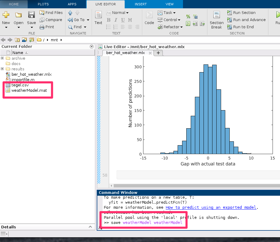
 5. To save the working model to be used later, copy and paste the following in the Command Window and then press Enter.
```matlab theme={null}
save weatherModel weatherModel
```
5. To save the working model to be used later, copy and paste the following in the Command Window and then press Enter.
```matlab theme={null}
save weatherModel weatherModel
```
 ### 5: Make predictions
You can use the model to predict the weather for next year. You’ll generate a table with next year’s dates and add randomly selected, historical precipitation and minimum temperature data to the table for those dates. This information helps the model make proper predictions.
1. Create a new **Section Break** in your Live Script.
2. Copy and paste the following to create a table with date and temperature input data.
```matlab theme={null}
todayDate = datetime('today');
daysIntoFuture = 365;
endDate = todayDate + days(daysIntoFuture);
predictedMaxTemps = table('Size', [daysIntoFuture+1 7], 'VariableTypes', {'datetime', 'double', 'double', 'double', 'double', 'double', 'double'}, 'VariableNames', berWeatherTbl.Properties.VariableNames);
x=1;
```
3. Copy and paste the following to loop through the next 20 days and populate the table.
```matlab theme={null}
for i=todayDate:endDate
[y, m, d] = ymd(i);
minTemps = berWeatherTbl.TMIN(berWeatherTbl.month == m & berWeatherTbl.day == d);
prcps = berWeatherTbl.PRCP(berWeatherTbl.month == m & berWeatherTbl.day == d);
curMinTemp = NaN;
[historicalRowCount z] = size(minTemps);
randomRow = randi([1 historicalRowCount]);
curMinTemp = minTemps(randomRow);
predictedMaxTemps.TMIN(x) = curMinTemp;
randomRow = randi([1 historicalRowCount]);
predictedMaxTemps.PRCP(x) = prcps(randomRow);
predictedMaxTemps.DATE(x) = i;
predictedMaxTemps.year(x) = y;
predictedMaxTemps.month(x) = m;
predictedMaxTemps.day(x) = d;
predictedMaxTemps.TMAX(x) = 0;
x = x+1;
end
head(predictedMaxTemps)
```
4. Click **Run Section**.
The result is a preview of the table with historical weather data that you can use for weather predictions. The predictions will be listed in the **TMAX** column of the table after the table is run through the model.
### 5: Make predictions
You can use the model to predict the weather for next year. You’ll generate a table with next year’s dates and add randomly selected, historical precipitation and minimum temperature data to the table for those dates. This information helps the model make proper predictions.
1. Create a new **Section Break** in your Live Script.
2. Copy and paste the following to create a table with date and temperature input data.
```matlab theme={null}
todayDate = datetime('today');
daysIntoFuture = 365;
endDate = todayDate + days(daysIntoFuture);
predictedMaxTemps = table('Size', [daysIntoFuture+1 7], 'VariableTypes', {'datetime', 'double', 'double', 'double', 'double', 'double', 'double'}, 'VariableNames', berWeatherTbl.Properties.VariableNames);
x=1;
```
3. Copy and paste the following to loop through the next 20 days and populate the table.
```matlab theme={null}
for i=todayDate:endDate
[y, m, d] = ymd(i);
minTemps = berWeatherTbl.TMIN(berWeatherTbl.month == m & berWeatherTbl.day == d);
prcps = berWeatherTbl.PRCP(berWeatherTbl.month == m & berWeatherTbl.day == d);
curMinTemp = NaN;
[historicalRowCount z] = size(minTemps);
randomRow = randi([1 historicalRowCount]);
curMinTemp = minTemps(randomRow);
predictedMaxTemps.TMIN(x) = curMinTemp;
randomRow = randi([1 historicalRowCount]);
predictedMaxTemps.PRCP(x) = prcps(randomRow);
predictedMaxTemps.DATE(x) = i;
predictedMaxTemps.year(x) = y;
predictedMaxTemps.month(x) = m;
predictedMaxTemps.day(x) = d;
predictedMaxTemps.TMAX(x) = 0;
x = x+1;
end
head(predictedMaxTemps)
```
4. Click **Run Section**.
The result is a preview of the table with historical weather data that you can use for weather predictions. The predictions will be listed in the **TMAX** column of the table after the table is run through the model.
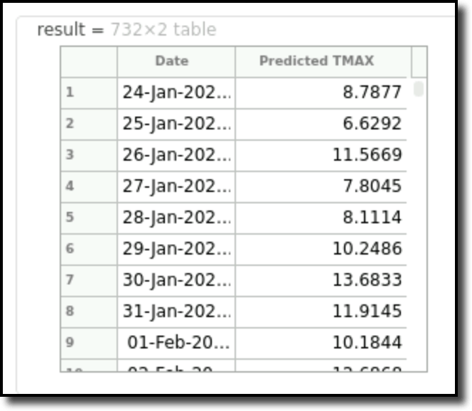
 5. To run the model, copy and paste the following into a new Section Break and run the Section.
```matlab theme={null}
yFit = weatherModel.predictFcn(predictedMaxTemps);
result = table(predictedMaxTemps.DATE, yFit, 'VariableNames', {'Date', 'Predicted TMAX'})
```
The following is an AI-driven weather prediction.
5. To run the model, copy and paste the following into a new Section Break and run the Section.
```matlab theme={null}
yFit = weatherModel.predictFcn(predictedMaxTemps);
result = table(predictedMaxTemps.DATE, yFit, 'VariableNames', {'Date', 'Predicted TMAX'})
```
The following is an AI-driven weather prediction.
 6. Copy and paste the following code, and then **Run Section** to draw this in another plot and count how many hot days will be forecasted:
```matlab theme={null}
figure
plot(result.Date, result.("Predicted TMAX"))
titleText = sprintf("%s%d%s", "Weather forecast for the next ", daysIntoFuture, " days in Berlin, Germany (\circC)");
title(titleText)
ylabel('Forecasted Daily High Temperature')
```
6. Copy and paste the following code, and then **Run Section** to draw this in another plot and count how many hot days will be forecasted:
```matlab theme={null}
figure
plot(result.Date, result.("Predicted TMAX"))
titleText = sprintf("%s%d%s", "Weather forecast for the next ", daysIntoFuture, " days in Berlin, Germany (\circC)");
title(titleText)
ylabel('Forecasted Daily High Temperature')
```
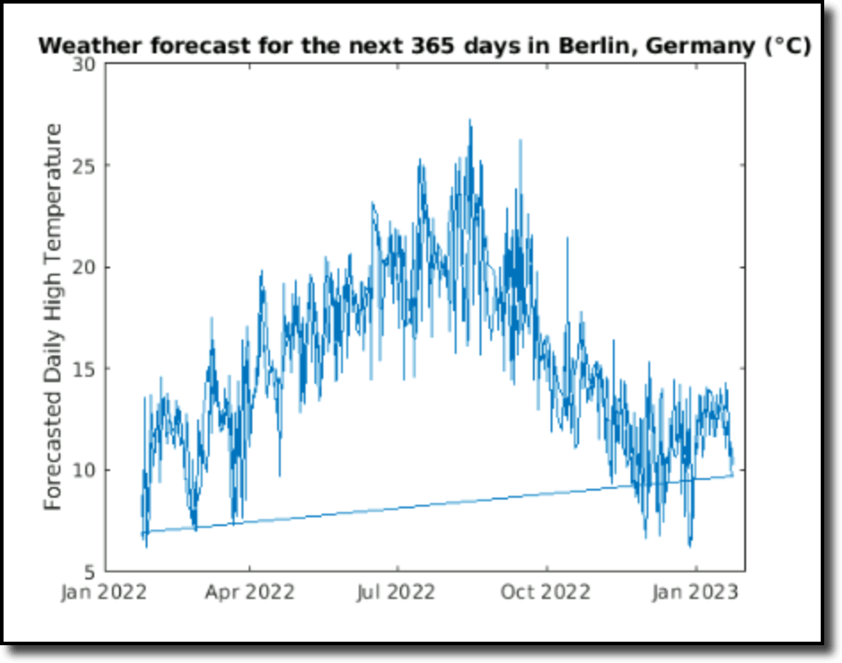 7. Copy and paste the following code, and then **Run Section** to predict how many hot days will happen during the next year.
```matlab theme={null}
hotWeatherDaysIdx = result(result.("Predicted TMAX") > hotDayThreshold, :);
height(hotWeatherDaysIdx)
```
The result on January 24, 2022 was a prediction of 0 hot days between January 2022 and February 2022. The results will vary based on the dates, data, and model used.
8. To export your model, in the Command Window, type the following to save it into a MAT file:
```matlab theme={null}
save weatherModel weatherModel
```
Anyone in your Domino project can load it later with the following command:
```matlab theme={null}
load weathermodel.mat
```
7. Copy and paste the following code, and then **Run Section** to predict how many hot days will happen during the next year.
```matlab theme={null}
hotWeatherDaysIdx = result(result.("Predicted TMAX") > hotDayThreshold, :);
height(hotWeatherDaysIdx)
```
The result on January 24, 2022 was a prediction of 0 hot days between January 2022 and February 2022. The results will vary based on the dates, data, and model used.
8. To export your model, in the Command Window, type the following to save it into a MAT file:
```matlab theme={null}
save weatherModel weatherModel
```
Anyone in your Domino project can load it later with the following command:
```matlab theme={null}
load weathermodel.mat
```