

Overview
AutoML is a Domino extension that enables data scientists and domain experts to build, evaluate, and deploy machine learning models through a streamlined, no-code interface. Powered by AutoGluon, AutoML automates the end-to-end model training pipeline - from data profiling and feature engineering through model selection, hyperparameter tuning, and ensembling - so you can go from raw data to a production-ready model in minutes. AutoML provides two primary workflows:- Data Exploration: Upload a dataset, review column statistics and distributions, examine correlations, assess data quality, and apply transformations before training.
- Model Training: Configure and run an AutoGluon training job that automatically trains multiple model types, ranks them on a leaderboard, and produces deployment-ready artifacts.
Get started
Prerequisites
- A Domino project with the AutoML extension enabled.
- A dataset in CSV or Parquet format (maximum file size: 550 MB).
- Alternatively, a file stored in a mounted Domino Dataset.
Installation
On Domino 6.3.0 and later, an administrator installs AutoML Studio from the Admin panel. See Install Domino Official Extensions. For earlier Domino versions, follow the manual install instructions in the AutoML_Extension repository, which also holds the source.Access AutoML
- Navigate to your Domino project.
- In the left sidebar, scroll down to the Extensions section.
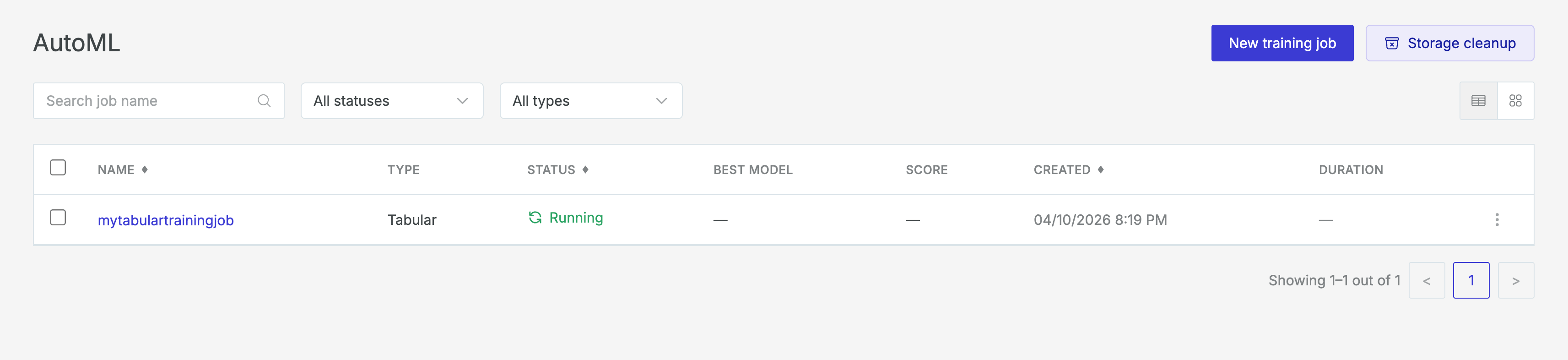
- Click AutoML.
Data exploration
The Data Exploration tool lets you analyze data quality, distributions, and correlations, and prepare transformations before training a model. To open it, click Explore Data from the AutoML landing page.Upload data
You can provide data in one of two ways:- Upload File: Drag and drop (or click to browse) a CSV or Parquet file. The maximum file size is 550 MB.
- Domino Dataset: Select a file from a mounted Domino Dataset already connected to your project.
Data preview
The Data Preview tab shows a sample of your raw data in table format. You can browse columns and rows to get a quick sense of the dataset’s structure and values. Use the Rows per page control to adjust how many rows are displayed at a time.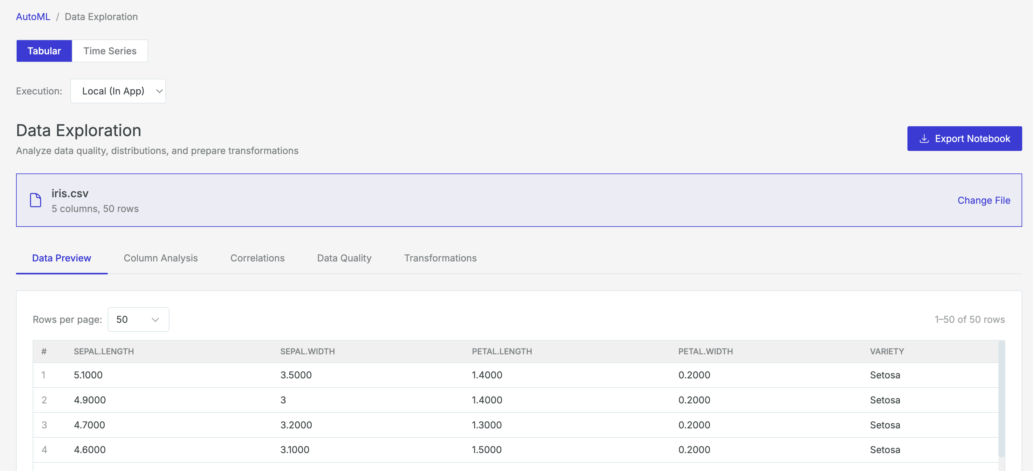
Column analysis
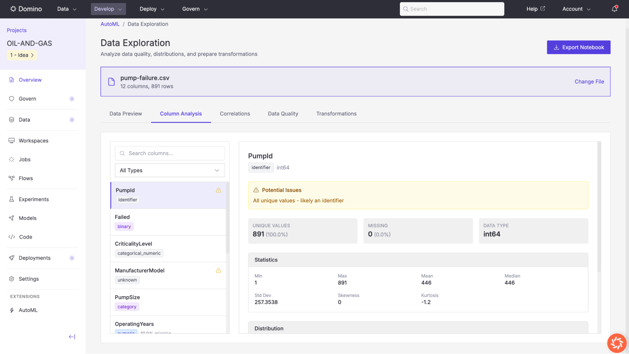
The Column Analysis tab provides detailed profiling information for each column in your dataset. Select a column from the list on the left to view its profile on the right. AutoML automatically detects each column’s semantic type, displayed as a colored tag beneath the column name. Detected types include:
Additional types are detected but displayed with default styling:
- email: Columns with email-related names
- phone: Columns with phone-related names
- url: Columns with URL-related names
- latitude/longitude: Geographic coordinate columns
-
percentage: Columns with percentage-related names (for example,
percent,pct,ratio,rate) -
name: Columns with name-related patterns (for example,
name,title,label) -
count: Columns with count-related names (for example,
count,num,qty,quantity)
-
Potential Issues: Warnings such as
High cardinality – may be an identifier,High missing rate, orConstant or near-constant column. - Unique Values: The count and percentage of distinct values.
- Missing: The count and percentage of null or missing entries.
-
Data Type: The underlying Pandas data type (for example,
int64,object,float64). -
Statistics: For numeric columns:
min,max,mean,median,standard deviation,skewness, andkurtosis. - Distribution: A histogram for numeric columns, or a bar chart of top values for categorical columns showing the count and percentage for each category.
Correlations
The Correlations tab displays a correlation matrix heatmap for all numeric columns in the dataset. Correlation values range from −1 (strong negative correlation) to +1 (strong positive correlation), with color coding to highlight the strength and direction of each relationship. Use the Min correlation slider to filter out weak correlations and focus on the strongest relationships. This view is helpful for identifying multicollinearity between features and understanding which variables are most associated with your target column.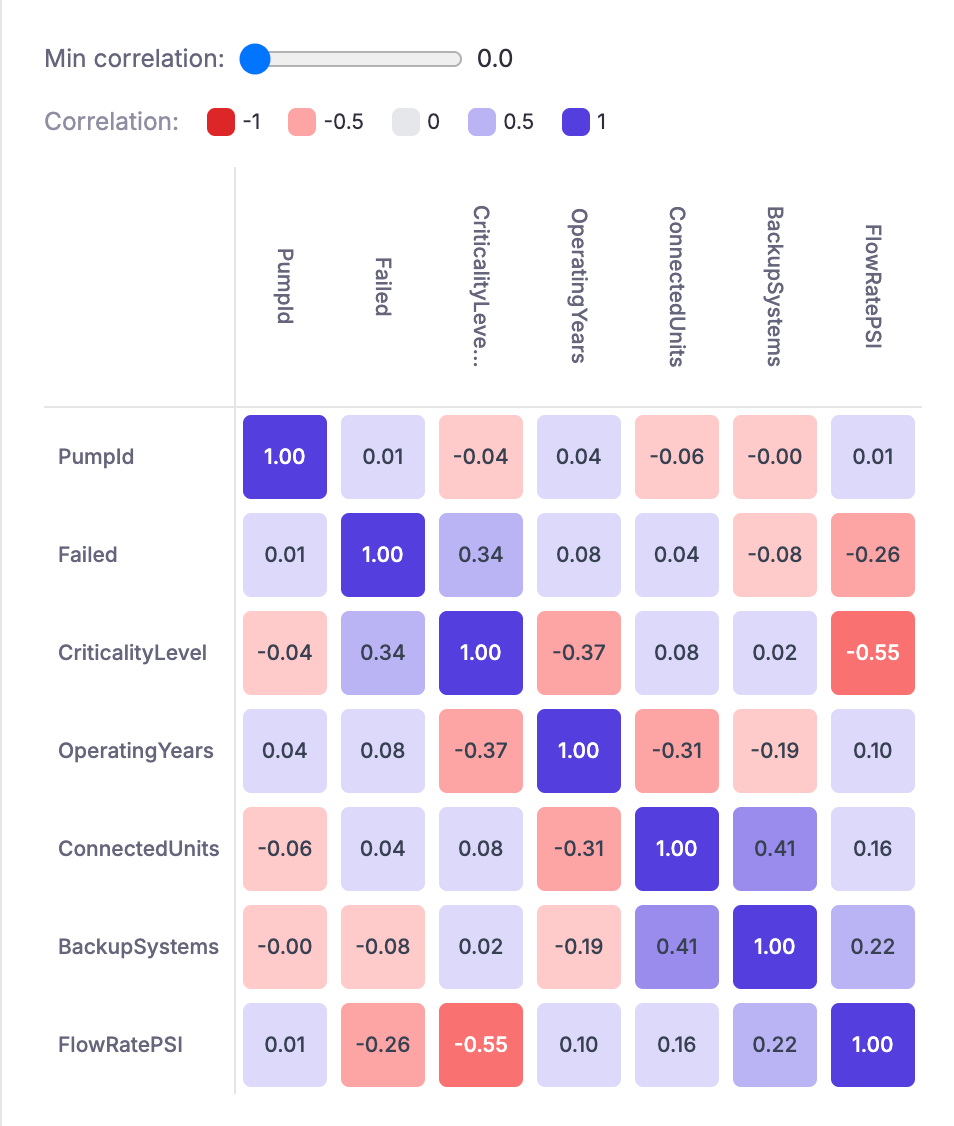
Data quality
The Data Quality tab gives you an at-a-glance assessment of your dataset’s readiness for model training. It includes the following sections:- Missing Values by Column: A horizontal bar chart showing the number and percentage of missing values for each column that has any. Columns are color-coded by severity: green for less than 5% missing, orange for 5–20%, yellow for 20–50%, and red for more than 50%.
- Missing Value Pattern: A compact visual representation of where missing values occur across columns, helping you identify whether missingness is concentrated or scattered.
-
Warnings: Issues that could affect training quality. For example,
Small dataset – consider using best_quality preset for better results. -
Recommendations: Actionable suggestions to improve model performance. These are tagged by priority (high or medium) and category (Target, Preprocessing). Examples include:
-
Potential binary classification targets (for example,
Failed,PumpSize). -
Potential multiclass classification targets (for example,
CriticalityLevel,ConnectedUnits,BackupSystems). -
Consider dropping or imputing columns with more than 30% missing values (for example,
WellSector).
-
Potential binary classification targets (for example,
Transformations
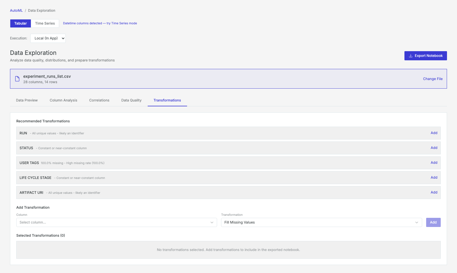
The Transformations tab lets you define preprocessing steps that are applied to the dataset before model training. AutoML analyzes your data and suggests recommended transformations based on detected issues. Recommended transformations AutoML may recommend transformations for columns with the following issues:-
Identifier columns: Columns where all values are unique and are likely row identifiers (for example,
PumpId). Recommended action: drop the column. -
High cardinality: Columns that may be identifiers due to a large number of unique values (for example,
ManufacturerModel). Recommended action: review and potentially drop. -
Missing values: Columns with a significant percentage of null values (for example,
OperatingYears at 19.9% missing). Recommended action: fill missing values. -
Extreme outliers: Numeric columns with extreme values detected (for example,
FlowRatePSI with 6.9% outliers). Recommended action: clip or remove outliers. -
High missing rate: Columns with a high percentage of missing data (for example,
WellSector at 77% missing). Recommended action: drop the column.
Fill Missing Values) from the dropdown controls at the bottom of the page.
All selected transformations appear in the Selected Transformations list. Transformations are included in the exported notebook and can be reviewed and modified in code.
Export a notebook
At any point during data exploration, you can click the Export Notebook button in the top-right corner to download a Jupyter notebook that contains all of your data profiling results and any transformations you have selected. This notebook can be opened in a Domino Workspace for further analysis or custom preprocessing.AutoML model training
AutoML model training uses AutoGluon to automatically train, tune, and rank multiple machine learning models. The training job wizard guides you through four steps: selecting your data source, choosing a model type, configuring training parameters, and reviewing your settings before launch. To begin, click New training job from the AutoML landing page.Step 1: Select a data source
Select the dataset you want to use for training. As with Data Exploration, you can either upload a CSV or Parquet file (up to 550 MB) or select a file from a mounted Domino Dataset. Once your file is loaded, click Continue to proceed.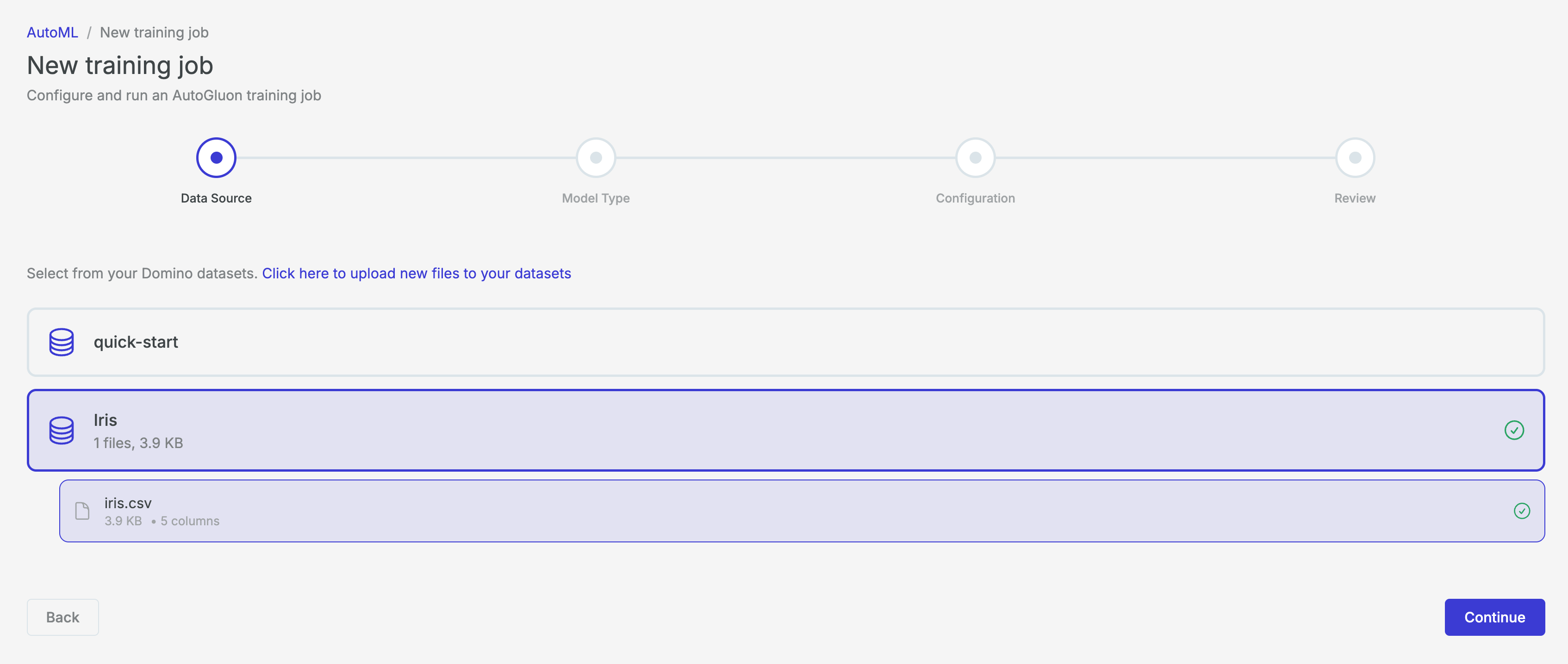
Step 2: Select a model type
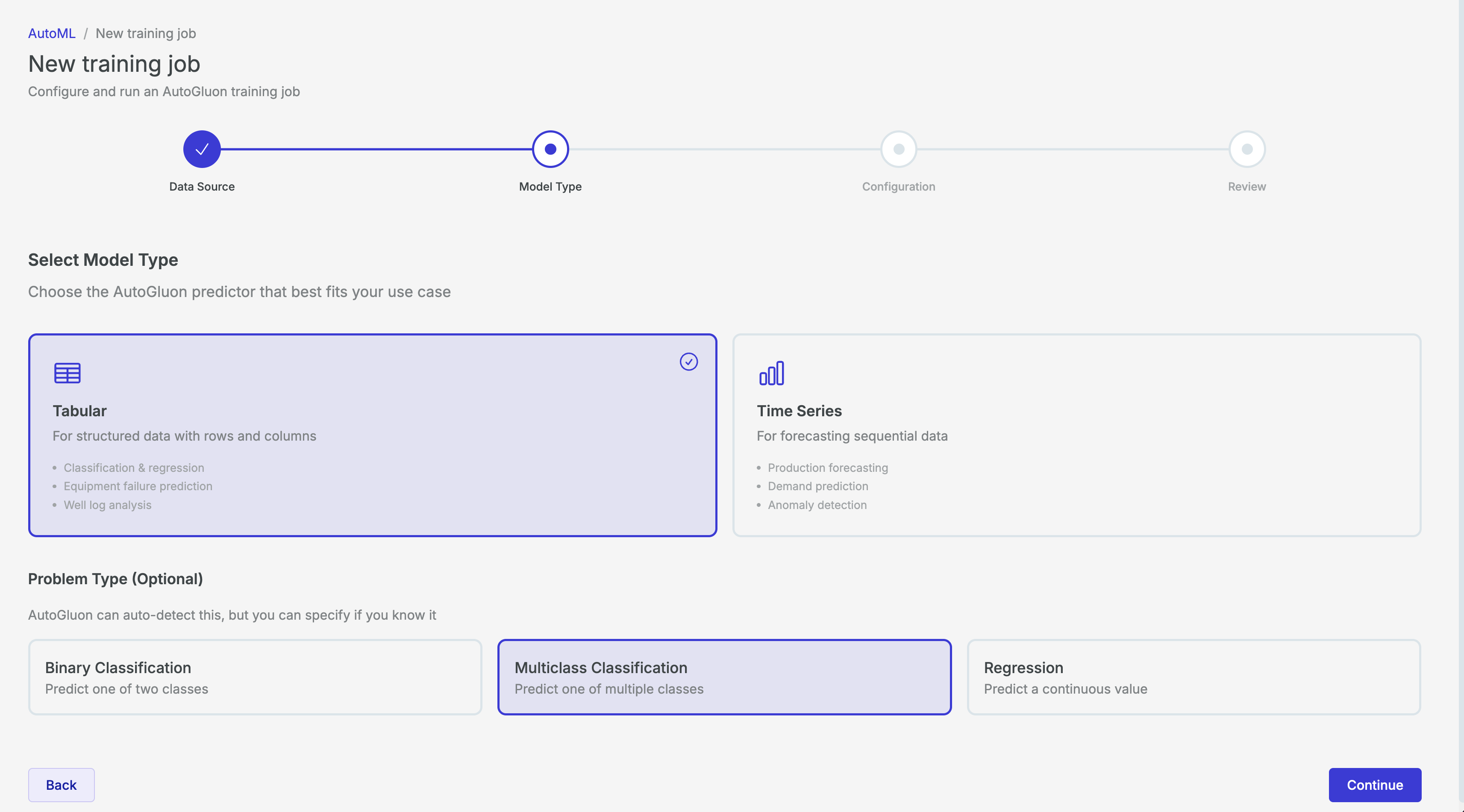
Choose the AutoGluon predictor that best fits your use case. Three model types are available:
Problem Type (Optional)
AutoGluon can auto-detect the problem type from your target column, but you can also specify it explicitly:
Click Continue to proceed to configuration.
Step 3: Configure training
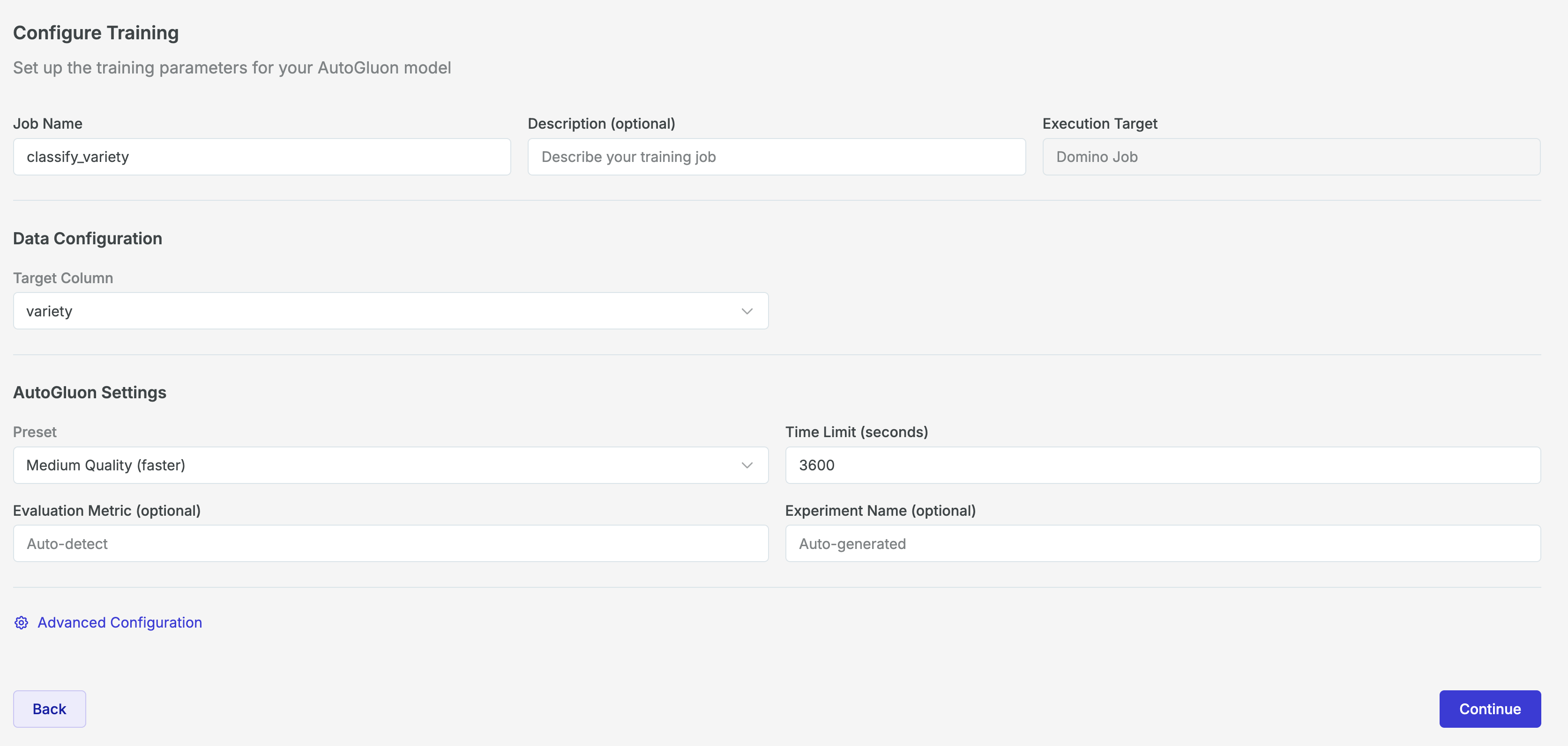
The configuration step lets you define your training job’s name, target column, and AutoGluon-specific settings.Basic configuration
AutoGluon settings
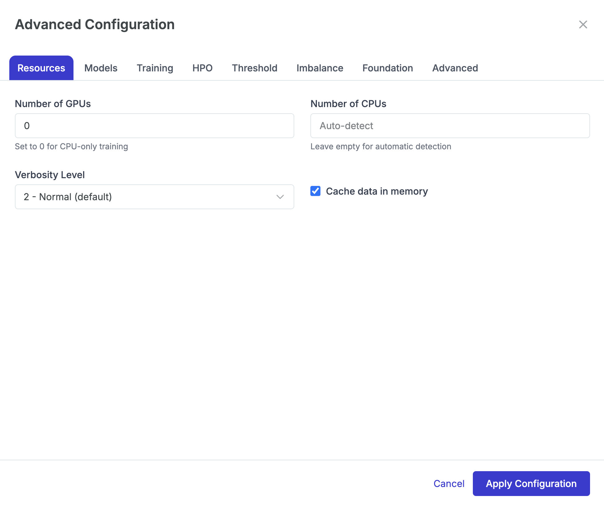
Advanced configuration
Click Advanced Configuration to access fine-grained controls organized across multiple tabs. Available tabs vary based on the selected model type.Tabs available for all model types
Tabs available for all model types
ResourcesConfigure compute resources allocated to the training job.
Tabs available for tabular models only
Tabs available for tabular models only
ModelsSelect or exclude specific model families from the training run.
TrainingFine-tune the training process.
Hyperparameter Optimization (HPO)Enable and configure hyperparameter tuning. When enabled, AutoGluon searches over hyperparameter combinations for each model family.
Per-Model Hyperparameters: Override default hyperparameters for specific model types (LightGBM, XGBoost, CatBoost, Neural Network) using JSON format.ThresholdFor binary classification tasks, optimize the decision threshold.
ImbalanceConfigure how AutoGluon handles class imbalance.
FoundationOptions for foundation model-based approaches.
AdvancedAdditional low-level AutoGluon parameters for experienced users.
Tabs available for time series models only
Tabs available for time series models only
Time SeriesConfigure time series-specific settings.
Tabs available for multimodal models only
Tabs available for multimodal models only
MultimodalConfigure multimodal-specific settings for combined image, text, and tabular data.
Step 4: Review and launch
Review all your selected settings on the summary screen. If everything looks correct, click Start Training to launch the job. You are taken to the training run’s overview page where you can monitor progress in real time.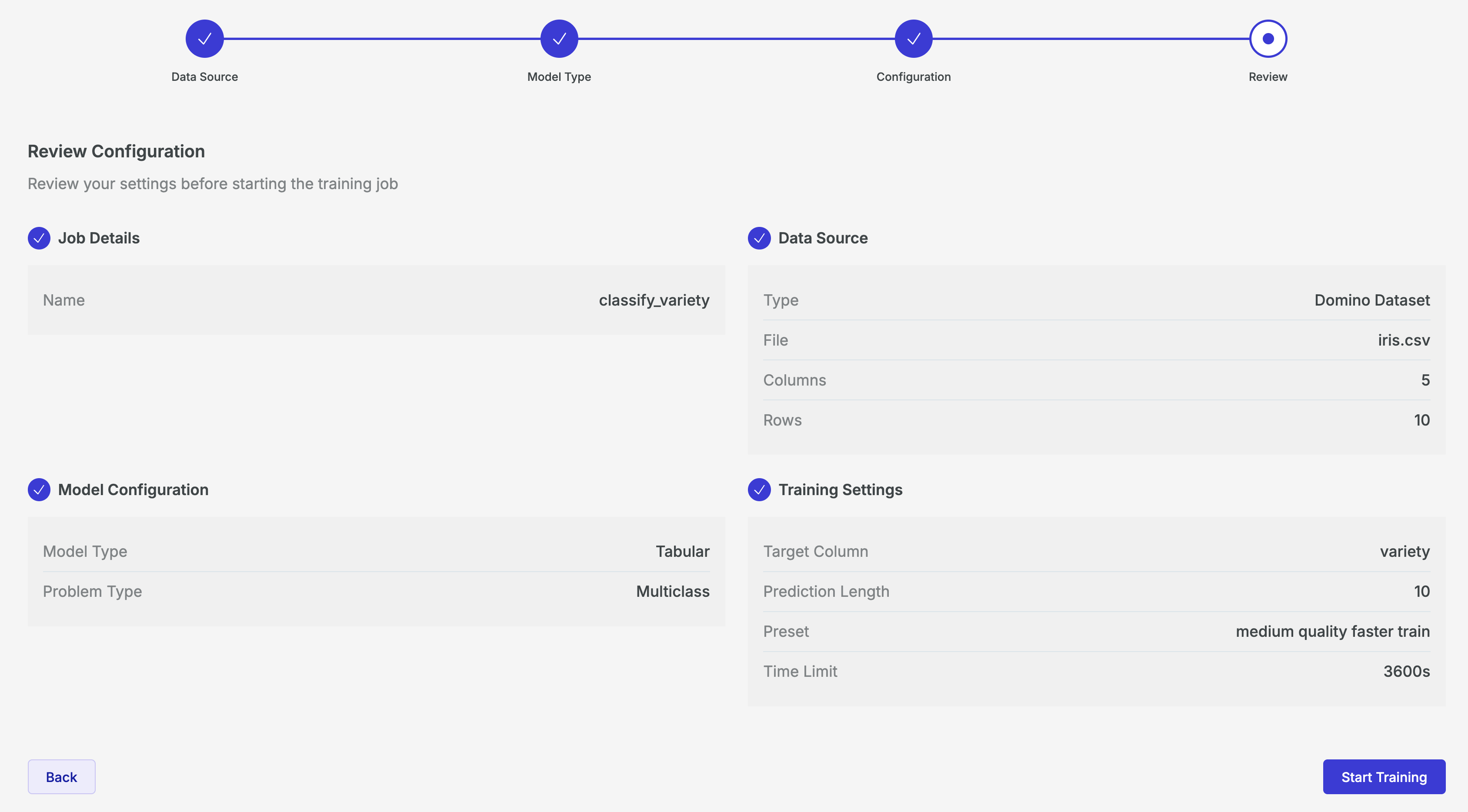
Training results
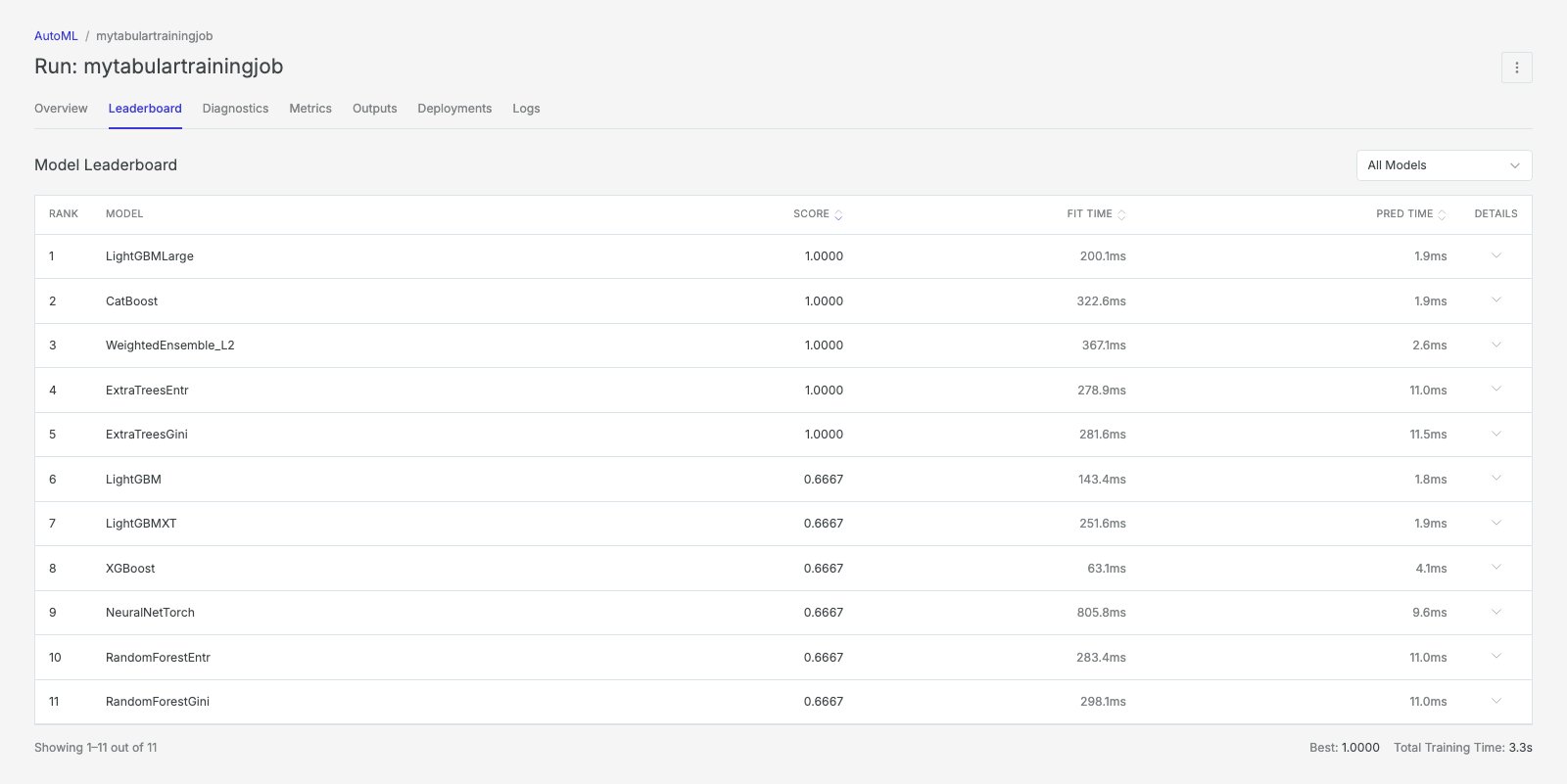
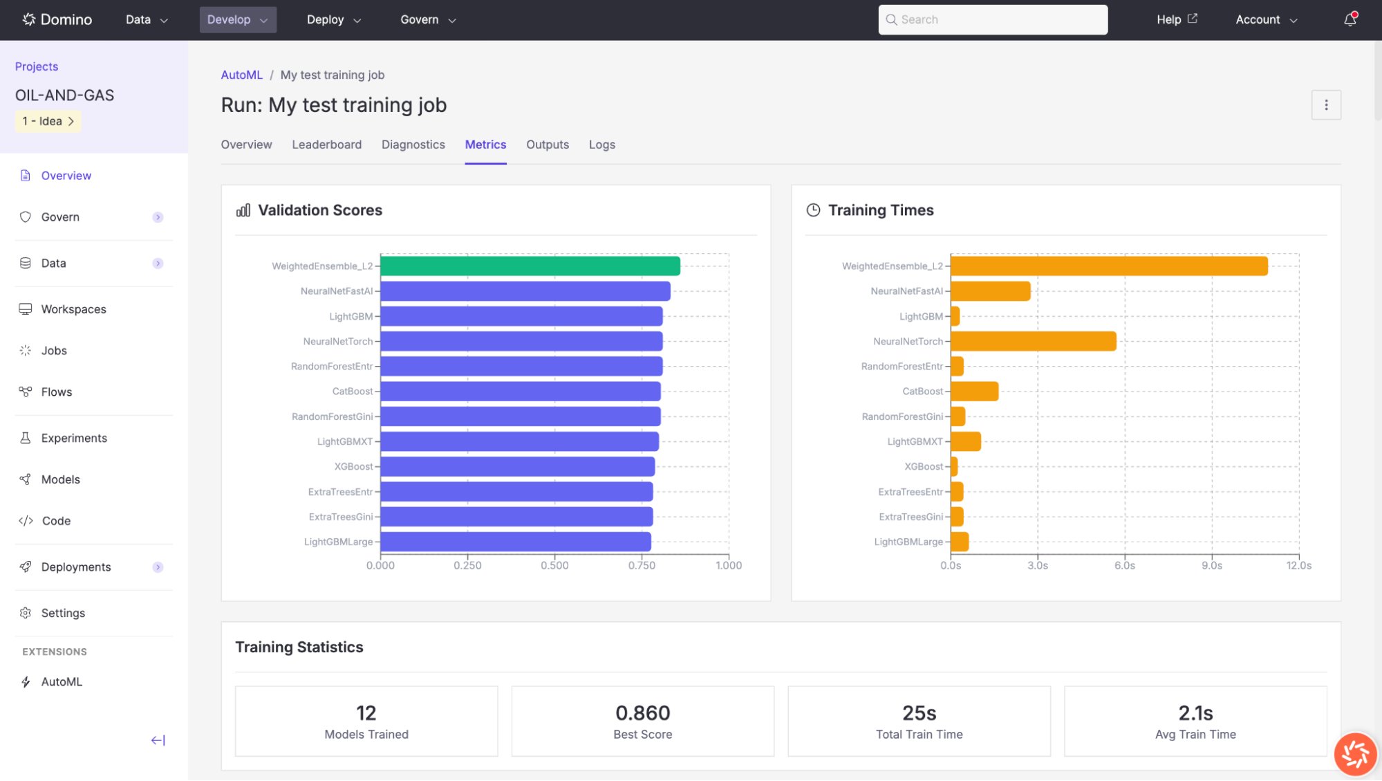
Once a training job is launched, its results page provides comprehensive information about the run’s progress and outputs. The results page is organized into several tabs: Overview, Leaderboard, Diagnostics, Metrics, Outputs, and Logs.- Overview
- Model Leaderboard
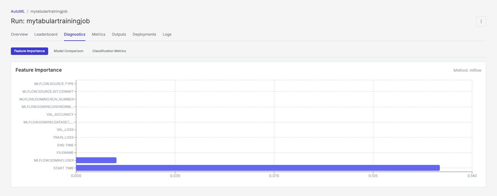
- Diagnostics
- Metrics
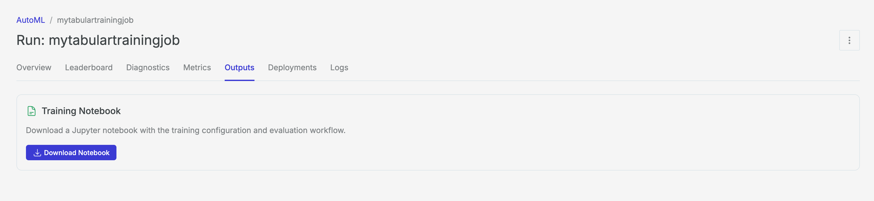
- Outputs
- Logs
- Forecast (Time Series Only)
The Overview tab displays the training job’s metadata and real-time progress. While the job is running, a progress bar shows the estimated completion percentage and a Cancel button is available to stop the run.The metadata table includes:
Deploy a model
After training is complete, you can deploy the best model directly from the AutoML interface.Export a deployment package
- Navigate to the Outputs tab of your completed training run.
- Verify the output directory path under Deployment Package.
- (Optional) Check Optimize for inference to reduce model size and improve prediction latency.
- Click Create Package.
Register a model
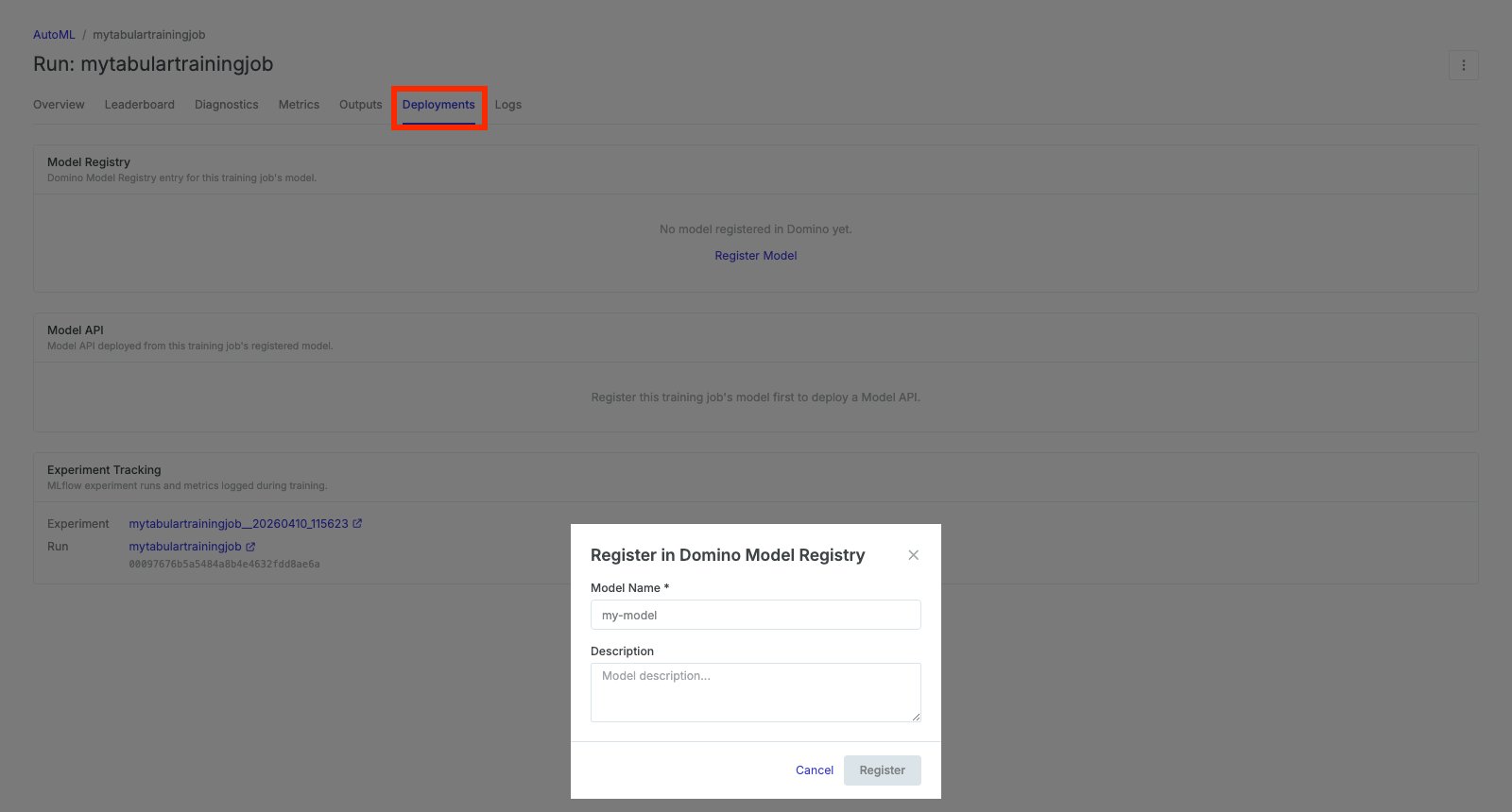
To register your model in Domino’s Model Registry for versioning, governance, and deployment:- Click the Register button in the top-right corner of the training results page.
- In the Deploy to Model Registry dialog, enter a Model Name.
-
Select the Model Type (for example,
Tabular). - Optionally add a description to document the model’s purpose and training context.
- Click Register to save the model to the registry.
Best practices
- Review data quality before training. Use the Data Exploration tool to inspect missing values, outliers, and column types. Address high-priority recommendations (especially dropping or imputing columns with more than 30% missing data) before starting a training job.
- Choose the right preset. The Medium Quality (Faster) preset is a good starting point for rapid iteration. Once you have identified a promising dataset and target, switch to Best Quality for production models, especially on smaller datasets where the additional training time yields meaningful improvements.
- Set an appropriate time limit. A longer time limit allows AutoGluon to train more models and explore more hyperparameter configurations. For initial exploration, 600–1800 seconds is often sufficient. For production runs, consider 3600 seconds or more.
- Exclude identifier columns. Columns with all unique values (flagged as identifiers) do not contribute meaningful signal and should be dropped before training. AutoML flags these in both Column Analysis and Recommended Transformations.
- Examine feature importance. After training, review the Feature Importance chart on the Diagnostics tab. If unimportant features dominate, consider removing them and retraining to reduce noise and improve generalization.
- Consider the prediction time trade-off. Ensemble models (for example, WeightedEnsemble_L2) typically achieve the best validation scores but may have higher inference latency. For real-time applications, compare leaderboard scores with prediction times and consider selecting a simpler model that meets your latency requirements. Use the exported notebook for reproducibility. Download the Training Notebook from the Outputs tab to preserve a complete record of your training configuration. This notebook can be re-run in a Domino Workspace and serves as the starting point for any custom modifications.